
# Install pak if not available
if (!requireNamespace("pak", quietly = TRUE)) {
  install.packages("pak")
}

# Student packages for rrcompendium project (Day 5)
dependencies <- c(
  "broom",
  "credentials",
  "devtools",
  "dplyr",
  "ggplot2",
  "ggthemes",
  "gt",
  "readr",
  "renv",
  "usethis",
  "benmarwick/rrtools"
)

pak::pak(dependencies)

# Install tinytex for PDF rendering
pak::pak("tinytex")
tinytex::install_tinytex()Creating a research compendium with rrtools
Research Compendia
Background
Research is increasingly computational
-
Code and data are important research outputs
- yet, we still focus mainly on curating papers.
-
Calls for openness
- stick: reproducibility crisis
- carrot: big rewards from working open
Yet we lag in conventions and technical infrastructure for such openness.
Enter the Research Compendium
The goal of a research compendium is to provide a standard and easily recognizable way for organizing the digital materials of a project to enable others to inspect, reproduce, and extend the research.
Three Generic Principles
-
Organize its files according to prevailing conventions:
- help other people recognize the structure of the project,
- supports tool building which takes advantage of the shared structure.
Separation of data, method, and output, while making the relationship between them clear.
Specify the computational environment that was used for the original analysis.
R community response
R packages can be used as a research compendium for organising and sharing files!
R package file system structure for reproducible research
Take advantage of the power of convention.
Make use of great package development tools.
See Ben Marwick, Carl Boettiger & Lincoln Mullen (2018) Packaging Data Analytical Work Reproducibly Using R (and Friends), The American Statistician, 72:1, 80-88, DOI: <10.1080/00031305.2017.1375986>
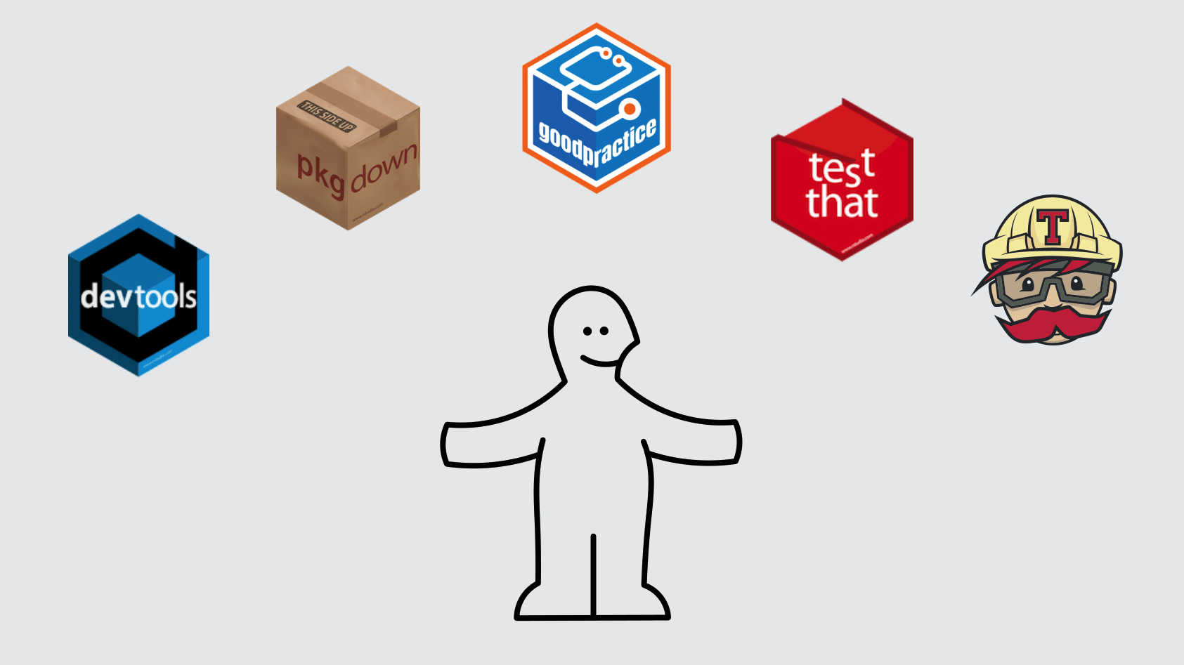
R Developer Tools
Leverage tools and functionality for R package development
- manage dependencies
- make functionality available
- document functionality
- validate functionality
- version control your project
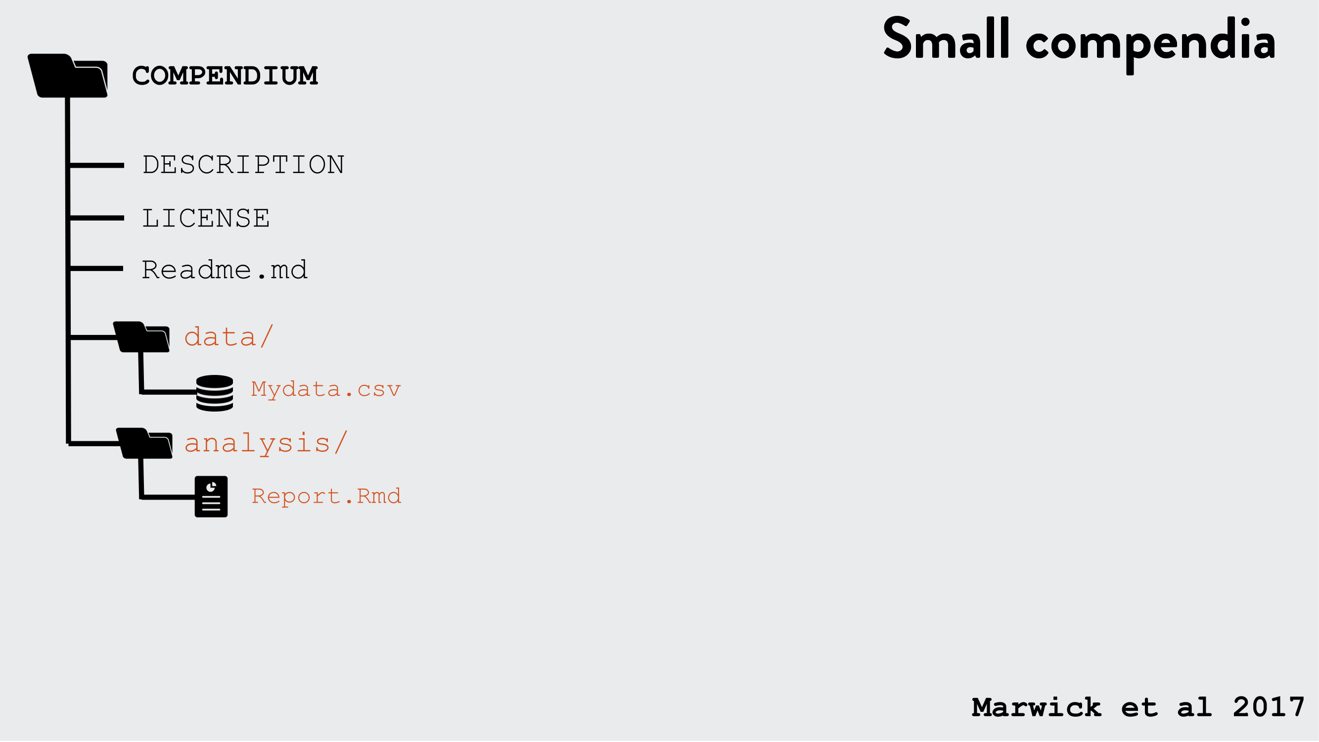
minimal analysis project
An
analysis/directory that contains R scripts (.R), notebooks (.qmd), and intermediate data.A
DESCRIPTIONfile that provides metadata about the compendium. Most importantly, it would list the packages needed to run the analysis. Would contain field to indicate that this is an analysis, not a package.
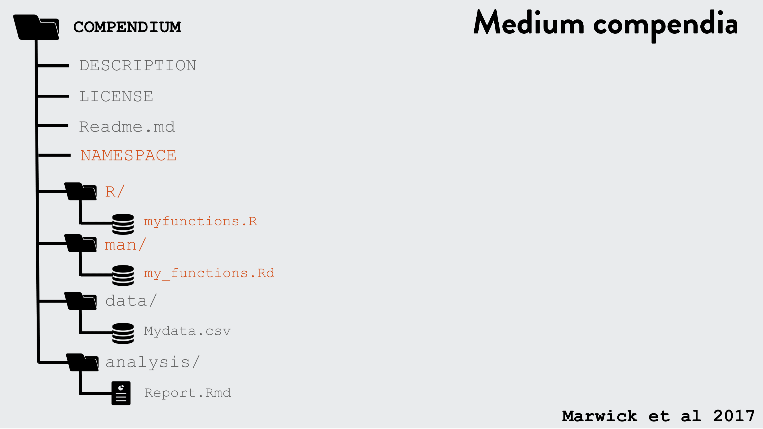
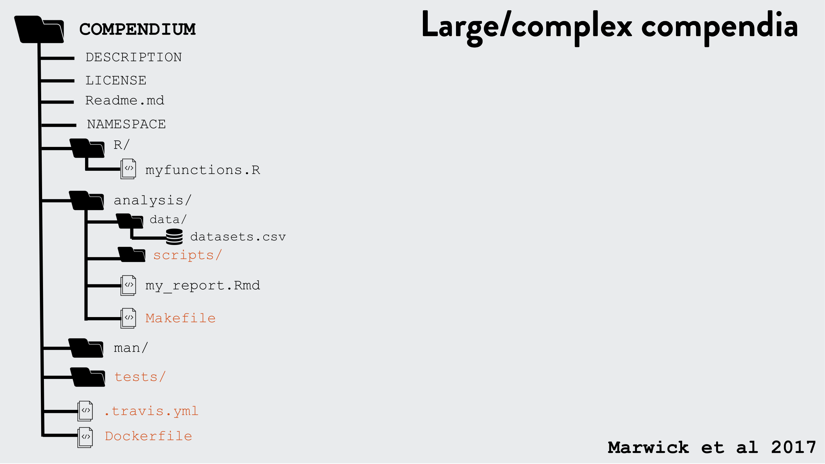
A reproducible analysis project might also contain:
An
R/directory which contains R files that provide high-stakes functions.A
data-raw/directory which contains raw data and the scripts that turn it into analytical data.A
data/directory which contains high-stakes analytical data.A
tests/directory that contains unit tests for the code and data.A
vignettes/directory that contains high-stakes reports.
Autogenerated components:
A
man/directory which contains roxygen2-generated documentation for the reusable functions and data.A
NAMESPACEfile (when the project includes reusable functions inR/) which declares exported and imported functions.Online documentation in a
docs/folder.
Start small and build as necessary
rrtools: Research Compendia in R
The goal of rrtools is to provide instructions, templates, and functions for making a basic compendium suitable for writing reproducible research with R.
rrtools builds on tools & conventions for R package development to
- organise files
- manage dependencies
- share code
- document code
- check and test code
rrtools extends and works with a number of R packages:
devtools: functions for package developmentusethis: automates repetitive tasks that arise during project setup and developmentQuarto: facilitates writing of Scientific and Technical Documents.
Practical: Create a Research Compendium
Practical Aims and Objectives
In this section we’ll use materials associated with a published paper (text, data and code) to create a research compendium around it.
By the end of the workshop, you should be able to:
Create a Research Compendium to manage and share resources associated with an academic publication.
Produce a reproducible manuscript from a single Quarto document.
Appreciate the power of convention!
Create your first reproducible research compendium
Let’s go ahead and create our first reproducible research compendium!
Copy rrcompendium Project
In our shared space click on the copy button next to the rrcompendium Project.
The project already has the rrtools package and all the necessary dependencies installed.
Installing required packages locally
If you are working locally, you would need to install the following packages starting with rrtools.
You might also need to install tinytex (if you get errors when rendering your qmd paper).
Fresh Posit Cloud project: re-do your git / GitHub setup
You’re starting in a brand-new Posit Cloud project, which means none of your git or GitHub configuration carries over from previous projects. Before we go any further, run:
# tell git who you are
usethis::use_git_config(
  user.name = "Your Name",
  user.email = "your.email@example.com"
)

# load your PAT into the credential store and current R session
credentials::set_github_pat()
See Configure git & GitHub for the full details.
Create compendium
Now that we’ve got a project to work in, let’s start by creating a blank research compendium for us to work in.
We use function rrtools::create_compendium().
Because we are already in the project we want to create the compendium in, we can just call the function without any arguments.
rrtools::create_compendium()But see below for information on how to create a compendium locally in a new directory.
Creating a Research Compendium in a new directory locally
Locally we could supply a path at which our compendium will be created. The final part of our path becomes the compendium name. Because the function effectively creates a package, only a single string of lowercase alpha characters is accepted as a name, for example, rrcompendium as the final part of our path.
To create rrcompendium on my desktop I might use:
rrtools::create_compendium("~/Desktop/rrcompendium")
R version 4.5.3 (2026-03-11) -- "Reassured Reassurer"
Copyright (C) 2026 The R Foundation for Statistical Computing
Platform: x86_64-pc-linux-gnu

R is free software and comes with ABSOLUTELY NO WARRANTY.
You are welcome to redistribute it under certain conditions.
Type 'license()' or 'licence()' for distribution details.

R is a collaborative project with many contributors.
Type 'contributors()' for more information and
'citation()' on how to cite R or R packages in publications.

Type 'demo()' for some demos, 'help()' for on-line help, or
'help.start()' for an HTML browser interface to help.
Type 'q()' to quit R.

> rrtools::create_compendium()
Creating the compendium in the current directory: /cloud/project
Creating the compendium in the current directory: /cloud/project
✔ Setting active project to "/cloud/project".
✔ Writing 'DESCRIPTION'.
Package: project
Title: What the Package Does (One Line, Title Case)
Version: 0.0.0.9000
Authors@R (parsed):
    * First Last <first.last@example.com> [aut, cre]
Description: What the package does (one paragraph).
License: MIT + file LICENSE
ByteCompile: true
Encoding: UTF-8
LazyData: true
Roxygen: list(markdown = TRUE)
RoxygenNote: 7.3.3
✔ Writing 'NAMESPACE'.
✔ The package project has been created
✔ The working directory is now /cloud/project

Next, you need to:  ↓ ↓ ↓
• Edit the DESCRIPTION file
• Add a license file (e.g. with usethis::use_mit_license(copyright_holder = 'Your Name'))
• Use other 'rrtools' functions to add components to the compendium
✔ Writing 'LICENSE'.
✔ Writing 'LICENSE.md'.
✔ Adding "^LICENSE\\.md$" to '.Rbuildignore'.

✔ Creating 'README.qmd' from template.
✔ Adding 'README.qmd' to `.Rbuildignore`.
• Modify 'README.qmd'
✔ Adding code of conduct.
✔ Creating 'CONDUCT.md' from template.
✔ Adding 'CONDUCT.md' to `.Rbuildignore`.
✔ Adding instructions to contributors.
✔ Creating 'CONTRIBUTING.md' from template.
✔ Adding 'CONTRIBUTING.md' to `.Rbuildignore`.
✔ Adding .binder/Dockerfile for Binder
✔ Creating '.binder'
✔ Creating '.binder/Dockerfile' from template.
✔ Adding '.binder/Dockerfile' to `.Rbuildignore`.
• Modify '.binder/Dockerfile'

✔ Adding 'here' pkg to Imports
✔ Creating 'analysis' directory and contents
✔ Creating 'analysis'
✔ Creating 'analysis/paper'
✔ Creating 'analysis/figures'
✔ Creating 'analysis/templates'
✔ Creating 'analysis/data'
✔ Creating 'analysis/data/raw_data'
✔ Creating 'analysis/data/derived_data'
✔ Creating 'analysis/supplementary-materials'
✔ Creating 'references.bib' from template.
✔ Creating 'paper.qmd' from template.

Next, you need to:  ↓ ↓ ↓ ↓
• Write your article/report/thesis, start at the paper.qmd file
• Add the citation style library file (csl) to replace the default provided here, see https://github.com/citation-style-language/
• Add bibliographic details of cited items to the 'references.bib' file
• For adding captions & cross-referencing in an qmd, see https://quarto.org/docs/authoring/cross-references.html
• For adding citations & reference lists in an qmd, see https://quarto.org/docs/authoring/footnotes-and-citations.html

Note that:
⚠ Your data files are tracked by Git and will be pushed to GitHub

✔ The working directory is now /cloud/project
Note
On Posit Cloud, after Writing 'NAMESPACE'. you will also see an interactive prompt:
! Overwrite pre-existing file project.Rproj?

1: No way
2: Absolutely not
3: For sure
This is because Posit Cloud projects already contain a project.Rproj file. Answer affirmatively (3) to overwrite.
Initiate git
With git identity configured, let’s initialise our compendium with .git.
We’ll commit the rrtools scaffold as-is so that, as we work through the workshop, the changes we make to each file show up clearly as diffs against this known baseline.
Note
In a real project, you’d more likely customise the template values first (your details in DESCRIPTION, your text in README.qmd, etc.) before making your initial commit, so your project history doesn’t open with placeholder boilerplate.
# initialise git and commit
usethis::use_git()
✔ Initialising Git repo
✔ Adding '.Rhistory', '.Rdata', '.httr-oauth', '.DS_Store', '.quarto' to '.gitignore'
There are 12 uncommitted files:
* '.binder/'
* '.gitignore'
* '.Rbuildignore'
* 'analysis/'
* 'CONDUCT.md'
* 'CONTRIBUTING.md'
* 'DESCRIPTION'
* 'LICENSE'
* 'LICENSE.md'
* 'NAMESPACE'
* ...
Is it ok to commit them?
1: No
2: Nope
3: Definitely
Selection: 3Let’s agree to commit the files and also to restart RStudio.
Let’s also change the default branch to the more modern convention of main instead of master. We can use usethis::git_default_branch_rename().
usethis::git_default_branch_rename()✔ Setting active project to "/cloud/project".
ℹ Local branch "master" appears to play the role of the
default branch.
✔ Moving local "master" branch to "main".
☐ Be sure to update files that refer to the default branch
by name.
Consider searching within your project for "master".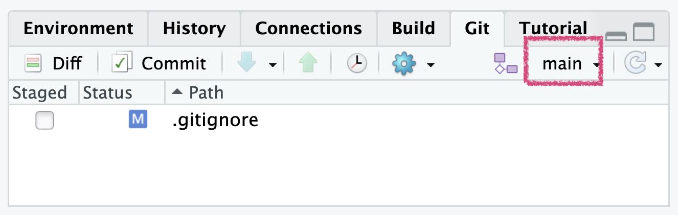
Inspect templates
rrtools::create_compendium() sets up a complete research compendium scaffold in one step. Together these files and directories provide everything we need to manage, install, and share both the functionality and the analysis associated with our project.
Let’s walk through what’s been created:
-
Package skeleton: turns the project into an installable R package, so dependencies and reusable functions can be managed using package conventions.
-
DESCRIPTION: package metadata (title, authors, description, license) and dependency management (Imports/Suggests). -
NAMESPACE: declares which functions are exported and imported. Auto-generated byroxygen2on build.
-
-
License files: make it explicit how others may reuse the code.
-
LICENSE: the canonical license file expected by R packages. -
LICENSE.md: a human-readable, GitHub-friendly version.
-
-
Project documentation: community-facing files for collaborators and users.
-
README.qmd: the landing page for the project; what people see first on GitHub. We render it toREADME.md. -
CONDUCT.md: code of conduct setting expectations for community behaviour. -
CONTRIBUTING.md: instructions for people who want to contribute.
-
-
analysis/: the full analysis tree, where the research itself lives. This is the part that distinguishes a research compendium from a vanilla R package.-
analysis/data/: analytical data, with subdirs forraw_data/andderived_data/. TheDO-NOT-EDIT-ANY-FILES-IN-HERE-BY-HANDmarker stresses that this is reproducible output, not source. -
analysis/figures/: figures generated by the analysis. -
analysis/paper/: the manuscript itself.-
paper.qmd: Quarto template for a reproducible manuscript. -
references.bib: bibliography file for citations.
-
-
analysis/supplementary-materials/: supplementary material that accompanies the paper. -
analysis/templates/: Lua filters, CSL style file, and Word/Rmd templates used when rendering the manuscript.
-
project.Rproj: the RStudio project file (this is the Posit Cloud default; it would be<pkgname>.Rprojlocally)..binder/Dockerfile: a Binder configuration for spinning up an interactive cloud copy of the compendium. We don’t go into Binder in this workshop, but it’s there for further exploration.
.
├── CONDUCT.md  <- .............................code of conduct
├── CONTRIBUTING.md <- .........................instructions for
|                                               contributors
├── DESCRIPTION <- .............................package metadata
|                                               dependency management
├── LICENSE <- .................................license files
├── LICENSE.md
├── NAMESPACE <- ...............................AUTO-GENERATED on build
├── README.qmd <- ..............................High level documentation
├── analysis
│   ├── data
│   │   ├── DO-NOT-EDIT-ANY-FILES-IN-HERE-BY-HAND
│   │   ├── derived_data
│   │   └── raw_data
│   ├── figures
│   ├── paper
│   │   ├── paper.qmd
│   │   └── references.bib
│   ├── supplementary-materials
│   └── templates
│       ├── author-info-blocks.lua
│       ├── journal-of-archaeological-science.csl
│       ├── pagebreak.lua
│       ├── scholarly-metadata.lua
│       ├── template.Rmd
│       └── template.docx
└── project.Rproj
Render analysis/paper/paper.qmd
Open the default paper.qmd that rrtools::create_compendium() placed in analysis/paper/ and click the Render button to see what the out-of-the-box reproducible manuscript template looks like. This is our starting point before we swap in the Elsevier template later.
Get session materials
Today we’ll be working with a subset of materials from the published compendium of code, data, and author’s manuscript:
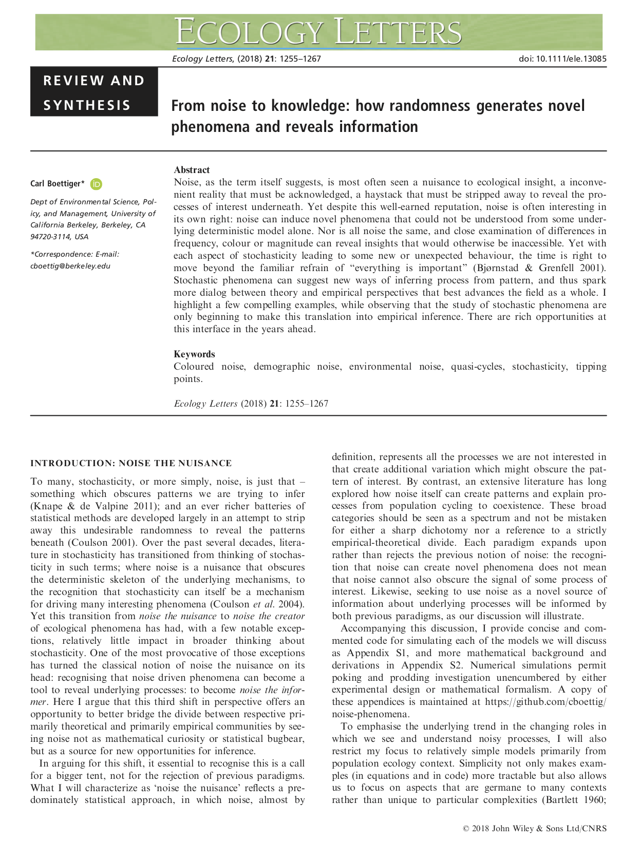
Carl Boettiger. (2018, April 17). cboettig/noise-phenomena: Supplement to: “From noise to knowledge: how randomness generates novel phenomena and reveals information” (Version revision-2). Zenodo. http://doi.org/10.5281/zenodo.1219780
accompanying the publication:
Carl Boettiger
. From noise to knowledge: how randomness generates novel phenomena and reveals information. Published in Ecology Letters, 22 May 2018 https://doi.org/10.1111/ele.13085
Create attic directory
Let’s first create a folder to download the materials into. It’s sometimes useful to have a folder to hold materials that are not formally part of the project (i.e. we will not commit these files to git). I like to call such folders attic, so let’s create such a folder
fs::dir_create("attic")Let’s also add the attic/ dir to .gitignore and .Rbuildignore (used to ignore files which should not be included as part of an installed R package) using usethis functions.
usethis::use_git_ignore("attic")
usethis::use_build_ignore("attic")
✔ Adding "attic" to .gitignore.
✔ Adding "^attic$" to .Rbuildignore.
Commit the changes to .gitignore and .Rbuildignore
Download materials
You can download the materials using usethis::use_course() and supplying a path to a destination folder to argument destdir. Let’s download everything into the attic/ folder.
usethis::use_course(url = "bit.ly/rrtools_wks", destdir = "attic")✔ Downloading from 'https://bit.ly/rrtools_wks'
Downloaded: 0.43 MB
✔ Download stored in 'attic/rrtools-wkshp-materials-master.zip'
✔ Unpacking ZIP file into 'rrtools-wkshp-materials-master/' (7 files extracted)
Shall we delete the ZIP file ('rrtools-wkshp-materials-master.zip')?
1: Yes
2: Nope
3: Absolutely not
Selection:
Enter an item from the menu, or 0 to exit
Selection: 1
✔ Deleting 'rrtools-wkshp-materials-master.zip'This will download everything we need from a GitHub repository as a .zip file, unzip it.
Inspect materials
The following files should now be contained in your attic/rrtools-wkshp-materials-master folder
├── README.md <- .......................materials README
├── analysis.R <- ......................analysis underlying paper
├── gillespie.csv <- ...................data
├── paper.pdf <- .......................LaTex pdf of the paper
├── paper.txt <- .......................text body of the paper
└── refs.bib <- ........................bibtex bibliographic file
In this workshop we’ll attempt a partial reproduction of the original paper using the materials we’ve just downloaded.
Now that we have the empty rrtools scaffold and the source materials side by side, our next step is to start populating the compendium: we’ll update the DESCRIPTION metadata to describe our project, then build up paper.qmd from the supplied text, data and analysis code.
Update DESCRIPTION file
The DESCRIPTION file is the metadata hub of the compendium, inherited from the R package conventions rrtools builds on. It captures who made the compendium, what it’s about, what license it carries, and which packages it depends on: the same single source of truth that R, GitHub and citation tools all read from.
For our compendium, the DESCRIPTION is where we record the title, authors, description and date of the project, and declare its dependencies so anyone can reconstruct the environment needed to reproduce the analysis. We’ll come back to the dependency side later; first let’s fill in the basic project details.
Let’s update some basic details in the DESCRIPTION file:
Package: project
Title: What the Package Does (One Line, Title Case)
Version: 0.0.0.9000
Authors@R:
    person("First", "Last", , "first.last@example.com", role = c("aut", "cre"))
Description: What the package does (one paragraph).
License: MIT + file LICENSE
ByteCompile: true
Encoding: UTF-8
LazyData: true
Roxygen: list(markdown = TRUE)
RoxygenNote: 7.3.3
Imports: here
Suggests: devtools,
    git2r
Package name
To work around the Posit Cloud limitation where all projects are called project, let’s correct the Package: field and rename our package to rrcompendium.
Package: rrcompendiumTitle
Let’s also give our compendium a descriptive title:
Title: Partial Reproduction of Boettiger Ecology Letters 2018;21:1255–1267
    with rrtools
Version
We don’t need to change the version now, but using semantic versioning is a useful way to track changes to our compendium over time. The default 0.0.0.9000 flags the project as early development: anything below 1.0.0 is considered pre-release, and the .9000 suffix is the R convention for “in-progress, not yet released”.
Bumping the version
Bump the version whenever you reach a point worth marking, like a snapshot accompanying a preprint or publication. You can use usethis::use_version() to do this for you.
Description
Let’s add a bit more detail about the contents of the compendium in the Description.
Description: This repository contains the research compendium of the
partial reproduction of Boettiger Ecology Letters 2018;21:1255–1267.
The compendium contains all data, code, and text associated with this
sub-section of the analysisDate
Add a Date field to the DESCRIPTION file to indicate when the compendium was created.
Date: 2026-05-01License
Finally, let’s update the license for the material we create with copyright holder details. We’ll continue using the MIT license already created (Note however that this only covers the code). We can do this with:
usethis::use_mit_license("Anna Krystalli")You’ll be asked twice whether to overwrite the existing LICENSE and LICENSE.md files (the placeholders created by rrtools::create_compendium()). Select the affirmative option both times so they’re replaced with the new versions that include your copyright details.
Overwrite pre-existing file 'LICENSE'?
1: No
2: Definitely
3: Not now
Selection: 2
✔ Writing 'LICENSE'
Overwrite pre-existing file 'LICENSE.md'?
1: Yup
2: Absolutely not
3: Not now
Selection: 1
✔ Writing 'LICENSE.md'This overwrites the current files LICENSE and LICENSE.md and updates the DESCRIPTION file, embedding our name in the details of the license.
Recap
We’ve finished updating our DESCRIPTION file! 🎉
It should look a bit like this:
DESCRIPTION
Package: rrcompendium
Title: Partial Reproduction of Boettiger Ecology Letters 2018;21:1255–1267
with rrtools
Version: 0.0.0.9000
Authors@R:
    person(given = "Anna",
           family = "Krystalli",
           role = c("aut", "cre"),
           email = "annakrystalli@googlemail.com",
           comment = c(ORCID = "0000-0002-2378-4915"))
Description: This repository contains the research compendium of the
    partial reproduction of Boettiger Ecology Letters 2018;21:1255–1267.
    The compendium contains all data, code, and text associated with this
    sub-section of the analysis
License: MIT + file LICENSE
ByteCompile: true
Encoding: UTF-8
LazyData: true
Roxygen: list(markdown = TRUE)
RoxygenNote: 7.3.3
Date: 2026-05-01
Imports: here
Suggests: devtools,
git2rand your project folder should contain:
.
├── CONDUCT.md
├── CONTRIBUTING.md
├── DESCRIPTION
├── LICENSE
├── LICENSE.md
├── NAMESPACE
├── README.qmd
├── analysis
│   ├── data
│   │   ├── DO-NOT-EDIT-ANY-FILES-IN-HERE-BY-HAND
│   │   ├── derived_data
│   │   └── raw_data
│   ├── figures
│   ├── paper
│   │   ├── paper.qmd
│   │   └── references.bib
│   ├── supplementary-materials
│   └── templates
│       ├── author-info-blocks.lua
│       ├── journal-of-archaeological-science.csl
│       ├── pagebreak.lua
│       ├── scholarly-metadata.lua
│       ├── template.Rmd
│       └── template.docx
├── attic
│   └── rrtools-wkshp-materials-master
│       ├── README.md
│       ├── analysis.R
│       ├── gillespie.csv
│       ├── paper.pdf
│       ├── paper.txt
│       └── refs.bib
└── project.Rproj
Commit your DESCRIPTION updates, then move on to preparing the compendium for sharing on GitHub
Create paper.qmd from template
When we first created our compendium, a paper.qmd file was created in the analysis/paper directory. This file is a template for a reproducible manuscript that we can use to write up our analysis and also serves to demonstrate how a reproducible paper should be set up.
However, the template is quite generic and we want to take advantage of the fact that Quarto offers templates for specific journals.
Given the original paper was published in Ecology Letters, an Elsevier journal, we’ll use the elsevier quarto template.
Delete current paper/ directory
First, let’s delete the current paper/ directory and its contents.
fs::dir_delete("analysis/paper")Create new paper.qmd from template
Next let’s move over to the Terminal and use the quarto CLI to create a new paper.qmd file from the elsevier template. When asked whether you trust the authors of the template, select Yes.
Terminal
quarto use template quarto-journals/elsevierQuarto templates may execute code when documents are rendered. If you do not
trust the authors of the template, we recommend that you do not install or
use the template.
? Do you trust the authors of this template (Y/n) › YesNext, you’ll be asked whether you want to create and use a subdirectory for the template rather than the root of the project. Respond with a Y.
Terminal
? Create a subdirectory for template? (Y/n) ›
❯ Use a subdirectory for the template rather than the current directory.
Finally, you’ll be asked to provide a name for the new directory the new paper.qmd will be created in. Specify: analysis/paper.
Terminal
? Directory name: › analysis/paperThe template requires the following changes to extensions:
Elsevier Journal Format [Install] 0.4.5 (formats)
? Would you like to continue (Y/n) › Yes
Preparing template files...
Found 1 extension.
[✓] Copying
[✓] Installing extensions...
[✓] Copying files...
Extensions installed:
- Elsevier Journal Format
Files created:
- bibliography.bib
- placeholder.png
- style-guide/1pseperateaug.pdf
- style-guide/1psingleauthorgroup.pdf
- style-guide/elsdoc.pdf
- style-guide/elsdoc.tex
- style-guide/elstest-1p.pdf
- style-guide/elstest-1pdoubleblind.pdf
- style-guide/elstest-3p.pdf
- style-guide/elstest-3pd.pdf
- style-guide/elstest-5p.pdf
- style-guide/jfigs.pdf
- style-guide/makefile
- style-guide/pdfwidgets.sty
- style-guide/rvdtx.sty
- paper.qmdThis creates the following files and directories in the analysis/paper directory:
analysis/paper
├── _extensions/
├── bibliography.bib
├── paper.qmd
├── placeholder.png
└── style-guide/
Commit changes to the project
Inspect paper.qmd
The paper.qmd file is a template for a reproducible manuscript that we can use to write up our analysis. It contains a lot of information about the features of the elsevier template and how to use it.
Let’s open the new paper.qmd file and take a look at the contents.
Render analysis/paper/paper.qmd
Click the Render button to see what the Elsevier template looks like out of the box, before we customise it.
Complete paper Front Matter
The front matter is the YAML header at the top of a Quarto document, sandwiched between a pair of --- separators. It captures metadata about the document (title, authors, abstract, keywords, bibliography, output format options, etc.) which Quarto uses both to render the document and to populate the manuscript with the bibliographic details a journal expects.
For a scientific paper, the front matter is where we record who wrote it, where they’re affiliated, what it’s about (title, abstract, keywords), what it cites, and how it should be formatted.
Tip
We covered the YAML header in more detail back in Front Matter & Markdown Basics. Refer back to that section if you need a refresher on YAML syntax and indentation.
Let’s start by completing the front matter of the paper.qmd file.
Most of the information we need (title, author, abstract, keywords) lives in the source paper itself, so before we start, open paper.txt from attic/rrtools-wkshp-materials-master/ and keep it side-by-side with paper.qmd to copy the relevant content across.
paper.txt contents
The file comes from the rrtools-wkshp-materials repository:
paper.txt
From noise to knowledge: how randomness generates novel phenomena and reveals information

Carl Boettiger

Dept of Environmental Science, Policy, and Management, University of California Berkeley, Berkeley CA 94720-3114, USA

cboettig@berkeley.edu


 # Abstract

  Noise, as the term itself suggests, is most often seen a nuisance to ecological insight, a inconvenient reality that must be acknowledged, a haystack that must be stripped away to reveal the processes of interest underneath. Yet despite this well-earned reputation, noise is often interesting in its own right: noise can induce novel phenomena that could not be understood from some underlying determinstic model alone.  Nor is all noise the same, and close examination of differences in frequency, color or magnitude can reveal insights that would otherwise be inaccessible.  Yet with each aspect of stochasticity leading to some new or unexpected behavior, the time is right to move beyond the familiar refrain of "everything is important" (Bjørnstad & Grenfell 2001).  Stochastic phenomena can suggest new ways of inferring process from pattern, and thus spark more dialog between theory and empirical perspectives that best advances the field as a whole. I highlight a few compelling examples, while observing that the study of stochastic phenomena are only beginning to make this translation into empirical inference.  There are rich opportunities at this interface in the years ahead.

# Keywords
Coloured noise, demographic noise, environmental noise, quasi-cycles, stochasticity, tipping points

# Introduction: Noise the nuisance

To many, stochasticity, or more simply, noise,
is just that -- something which obscures patterns we are trying to infer (Knape & de Valpine 2011); and an ever richer batteries of statistical methods are developed largely in an attempt to strip away this undesirable randomness to reveal the patterns beneath (Coulson 2001).  Over the past several decades, literature in stochasticity has transitioned from thinking of stochasticity in such terms; where noise is a nuisance that obscures the deterministic skeleton of the underlying mechanisms, to the recognition that stochasticity can itself be a mechanism for driving many interesting phenomena (Coulson et al. 2004).  Yet this transition from noise the nuisance to noise the creator of ecological phenomena has had, with a few notable exceptions, relatively little impact in broader thinking about stochasticity.  One of the most provocative of those exceptions has turned the classical notion of noise the nuisance on its head: recognizing that noise driven phenomena can become a tool to reveal underlying processes: to become noise the informer.  Here I argue that this third shift in perspective offers an opportunity to better bridge the divide between respective primarily theoretical and primarily empirical communities by seeing noise not as mathematical curiosity or statistical bugbear, but as a source for new opportunities for inference.


In arguing for this shift, it essential to recognize this is a call for a bigger tent, not for the rejection of previous paradigms.  What I will characterize as 'noise the nuisance' reflects a predominately statistical approach, in which noise, almost by definition, represents all the processes we are not interested in that create additional variation which might obscure the pattern of interest.  By contrast, an extensive literature has long explored how noise itself can create patterns and explain processes from population cycling to coexistence.  These broad categories should be seen as a spectrum and not be mistaken for either a sharp dichotomy nor a reference to a strictly empirical-theoretical divide.  Each paradigm expands upon rather than rejects the previous notion of noise: the recognition that noise can create novel phenomena does not mean that noise cannot also obscure the signal of some process of interest.  Likewise, seeking to use noise as a novel source of information about underlying processes will be informed by both previous paradigms, as our discussion will illustrate.

Numerical simulations permit poking and prodding investigation unencumbered by either experimental design or mathematical formalism.

The code and data for the simulations in this paper are maintained at <https://github.com/cboettig/noise-phenomena>.

To emphasize the underlying trend in the changing roles in which we
see and understand noisy processes, I will also restrict my focus
to relatively simple models primarily from population ecology context.
Simplicity not only makes examples (in equations and in code) more
tractable but also allows us to focus on aspects that are germane to many
contexts rather than unique to particular complexities (Bartlett 1960; Levins
41 1966).

Nevertheless, that complexity matters -- few themes have been better
emphasized in the theoretical literature (Bjørnstad & Grenfell 2001).  Both
the foundational literature and recent research continue to echo the
theme of understanding the impact different real world complexities
have in stochastic dynamics.  As such, we will
rely on both textbooks and recent reviews to provide a proper treatment
of these issues, and focus on broader trends.

This review is structured into three sections: Origins of noise, emergent
phenomena, and noise-driven inference.  The first section lays the conceptual groundwork we will need, while also highlighting a shift to more and more mechanistically rooted descriptions of noise.  We will see where the common formulation of "deterministic skeleton plus noise term" comes from, how it  is best justified, and when it breaks down.  The second section introduces noise the creator, showing examples of ecological phenomena generated by stochasticity.  These examples will be familiar to most specialists but illustrate a different way of thinking than held by most ecologists, where noise is only a nuisance to be filtered or averaged out.  The third and final section, noise the informer, turns these examples back-to-front, asking what noise can tell us about a system: such as its underlying resilience or stability, or the approach of a catastrophic shift. Examples are fewer here, and have largely yet to benefit from the introduction of either the rigorous theorems or more complex models so plentiful in the previous sections.  Yet the promise of prediction, of early warning signs before tipping points, have spurred broad interest in such noise-based inference. This review is a call to both deepen the connection to mechanism and better formalize this thinking, but also look more broadly into other ways in which noisy phenomena can help inform and predict underlying processes.


## Demographic stochasticity

Demographic stochasticity refers to fluctuations in population sizes
or densities that arise from the fundamentally discrete nature of
individual birth and death events.  Demographic stochasticity is a
particularly instructive case for illustrating a mechanism for how
noise arises as an aggregate description from a lower-level mechanistic
process.  We summarize the myriad lower-level processes that
mechanistically lead to the event of a 'birth' in the population
as a probability: In a population of N identical individuals at
time t, a birth occurs with probability b_t(N_t) (_i.e._ a rate
that can depend on the population size, N), which increases the
population size to N+1. Similarly, death events occur with probability
d_t(N_t), decreasing the population size by one individual, to N-1.  Assuming
each of these events are independent, this is a state-dependent
Poisson process. The change in the probability of being in state
N is given by the sum over the ways to enter the state, minus the
ways to leave the state: a simple expression of probability balance
known as the master equation (Kampen 2007).  Note that in general
this approach is equally applicable to stochastic transitions of any sort,
not just step sizes of +/- 1 and not just birth and death events, but
can include transitions between stage classes or trait values, including
mutations to continuously-valued traits in evolutionary dynamics (e.g. Boettiger et al. 2010).


The  Gillespie (1977) provides an exact algorithmcfor simulating demographic stochasticity at an individual level.

The algorithm is a simple and direct implementation of the master equation, progressing in random step sizes determined by the waiting time until the next event. Free from both the approximations and mathematical complexity, the Gillespie algorithm is an interesting example of where we rely on a numerical implementation to check the accuracy of an analytic approximation, even in the case of simple models such as we will discuss.  Though the  algorithm is often maligned as numerically demanding, it can be run much more effectively even on large models on today's computers than when it was first developed in the 70s, and remains an underutilized approach for writing simple and approximation-free^[that is, free from the approximation made by SDE models as we see in the van Kampen example.  All models are, of course, only approximations.] stochastic ecological models.


As our objective is to tie the origins of noise more closely to biological
processes, it will be helpful to make the notion of a master equation concrete with a specific example.  We will focus on the classic case of Levins (1969) patch model, to illustrate the Gillespie algorithm and the van Kampen system size expansion

\begin{align}
\frac{\mathrm{d} n}{\mathrm{d} t} = \underbrace{c n \left(1 - \frac{n}{N}\right)}_{\textrm{birth}} - \underbrace{e n}_{\textrm{death}}, \label{levins}
\end{align}

where n individuals compete for a
finite number of suitable habitats N.  Individuals die a constant
rate e, and produce offspring at a constant rate c who then
have a probability of colonizing an open patch that is simply
proportional to the fraction of available patches, 1 - n/N.


Figure 1 shows the results of two exact SSA simulations of the classic patch model of Levins (1969).

# Conclusions

This review has explored three paradigms in how noise is viewed throughout the ecological literature, which I have dubbed respectively: noise the nuisance, noise the creator, and noise the informer.  Noise can be seen as a nuisance almost by definition: in examining the origins of noise, we have seen how stochasticity is introduced not because ecological processes are random in some fundamental sense, but rather, because those processes are influenced by a complex combination of forces we do not model explicitly.  In this view, noise captures all that additional variation that is separate from the process of interest, and a rich array of statistical methods allow us to separate the one from the other in observations and experiments.  By examining the origins of noise, we have seen that despite the complex ways in this noise can enter a model, that a Gaussian white-noise approximation (Kampen 2007; Black & McKane 2012) is often appropriate given a limit of a large system size -- a fact often invokedn implicitly but rarely derived explicitly from the theorems of Kurtz (1978) and others.

In this context, noise does not act to create phenomena of interest directly. The sudden transitions we seek to anticipate are still explained by the deterministic part of the model -- bifurcations. But nor is noise a nuisance that merely cloaks this deterministic skeleton from plain view: rather, it becomes a novel source of information that would be inaccessible from a purely deterministic approach.  I believe more examples of how noise can inform on underlying processes is possible, but will require greater dialog between these world views.


# Acknowledgements

The author acknowledges feedback and advice from the editor,
Tim Coulson and two anonymous reviewers. This work was supported in
part by  USDA National Institute of Food and Agriculture, Hatch
project CA-B-INS-0162-H.

# References


# Figure 1: Population dynamics from a Gillespie simulation of the Levins model with large (N=1000, panel A) and small (N=100, panel B) number of sites (blue) show relatively weaker effects of demographic noise in the bigger system. Models are otherwise identical, with e = 0.2 and c = 1 (code in appendix A). Theoretical predictions for mean and plus/minus one standard deviation shown in horizontal re dashed lines.
Add abstract and keywords
Next, let’s replace the abstract and keywords fields with the following.
abstract: |
  Noise, as the term itself suggests, is most often seen a nuisance to ecological insight, a inconvenient reality that must be acknowledged, a haystack that must be stripped away to reveal the processes of interest underneath. Yet despite this well-earned reputation, noise is often interesting in its own right: noise can induce novel phenomena that could not be understood from some underlying determinstic model alone.  Nor is all noise the same, and close examination of differences in frequency, color or magnitude can reveal insights that would otherwise be inaccessible.  Yet with each aspect of stochasticity leading to some new or unexpected behavior, the time is right to move beyond the familiar refrain of "everything is important" (Bjørnstad & Grenfell 2001).  Stochastic phenomena can suggest new ways of inferring process from pattern, and thus spark more dialog between theory and empirical perspectives that best advances the field as a whole. I highlight a few compelling examples, while observing that the study of stochastic phenomena are only beginning to make this translation into empirical inference.  There are rich opportunities at this interface in the years ahead.
keywords:
  - Coloured noise
  - demographic noise
  - environmental noise
  - quasi-cycles
  - stochasticity
- tipping pointsComplete paper body
Clear template content and paste text
Next, let’s clear the template body contents (everything outside the YAML Front Matter header) and paste the main text from paper.txt.
Copy everything between and including the # Introduction: ... and ## References sections in paper.txt and paste it into the paper.qmd file, below the YAML Front matter header.
Add Mathematical Notation
Through the ## Demographic stochasticity section of the paper, there is discussion of simulation parameters that in the original paper are formatted using mathematical notation. To format such in-line text using such notation, surround it with $ dollar signs.
Here’s an example of what that looks like in paper.qmd:
 We summarize the myriad lower-level processes that
mechanistically lead to the event of a 'birth' in the population
as a probability: In a population of $N$ identical individuals at
time t, a birth occurs with probability $b_t(N_t)$ (_i.e._ a rate
that can depend on the population size, $N$), which increases the
population size to $N+1$. Similarly, death events occur with probability
$d_t(N_t)$, decreasing the population size by one individual, to $N-1$.
And what it looks like when rendered:
We summarize the myriad lower-level processes that mechanistically lead to the event of a ‘birth’ in the population as a probability: In a population of \(N\) identical individuals at time t, a birth occurs with probability \(b_t(N_t)\) (i.e. a rate that can depend on the population size, \(N\)), which increases the population size to \(N+1\). Similarly, death events occur with probability \(d_t(N_t)\), decreasing the population size by one individual, to \(N-1\).
Read through that section and format any mathematical notation accordingly.
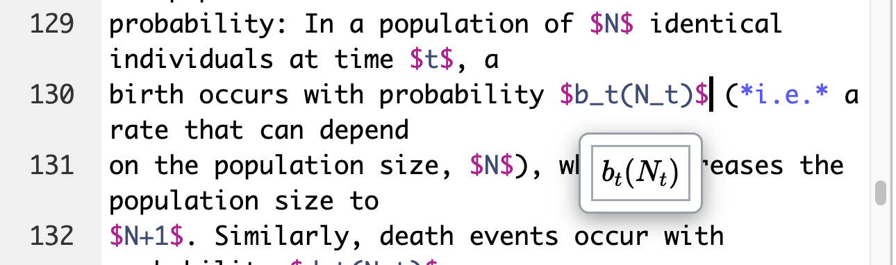
Previewing math notation as you type
You don’t need to render the full document to check your math. In the Source editor, RStudio shows a small popup preview of the rendered notation as you hover over or edit a $...$ expression:
In the Visual editor, the same notation is rendered inline directly in the text, so the document reads much like the final manuscript:
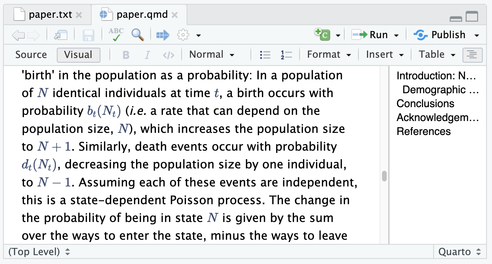
Either mode is a quick way to sanity-check your equations as you go.
Render analysis/paper/paper.qmd
Click the Render button to see the full body text in place with the equations correctly typeset. The flat citations in the text will still appear unformatted at this stage; we’ll deal with those next.
Update references
Quarto turns flat in-text markers into properly formatted, linked citations and an auto-generated References section at the bottom of the manuscript, all driven from a single bibliography file:
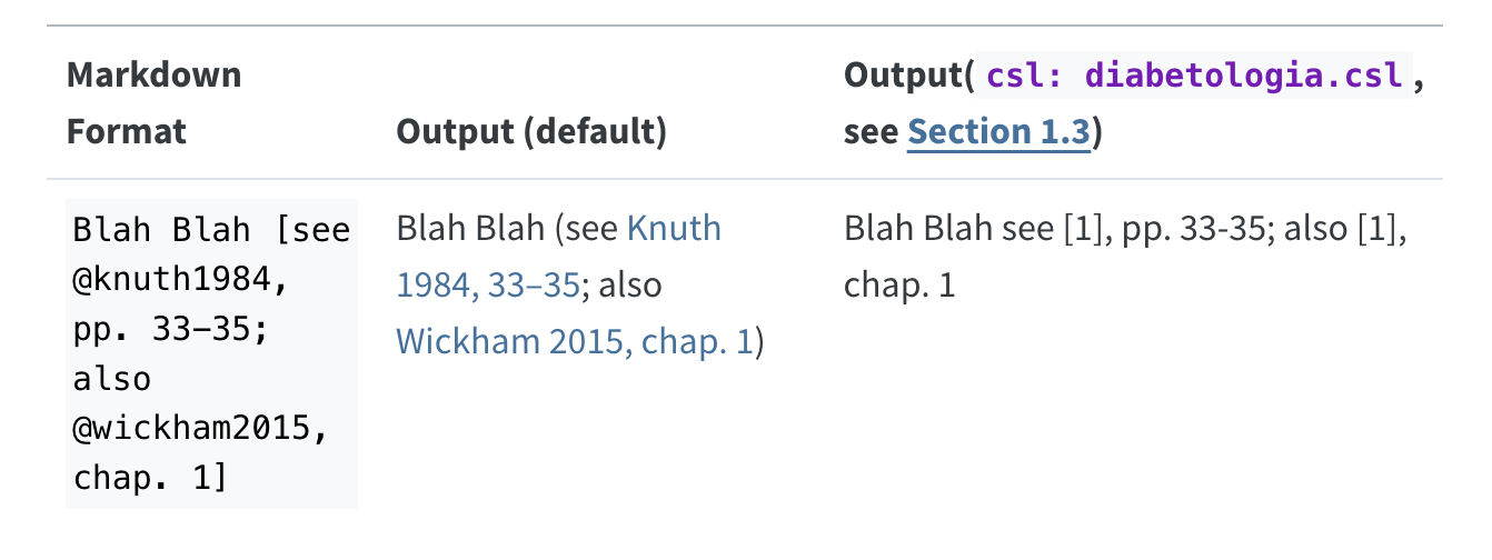
Next we’ll replace the flat citations in the text with real linked citations which can be used to auto-generate formatted in-line citations and the references section.
Add bibliography
First, let’s copy refs.bib from the downloaded materials into analysis/paper so it sits alongside paper.qmd:
fs::file_copy(
  "attic/rrtools-wkshp-materials-master/refs.bib",
  "analysis/paper"
)
Then, in the YAML Front Matter of paper.qmd, replace the bibliography field with the following to point at it:
bibliography: refs.bibInsert citation cross-references
Firstly, to use the interactive citation features in Quarto, we need to move over to the Visual editor.
Inserting citations interactively in the Visual editor
The easiest way to add citations is to use Insert > Citation… (⌘⇧F8 on macOS, Ctrl+Shift+F8 on Windows/Linux):
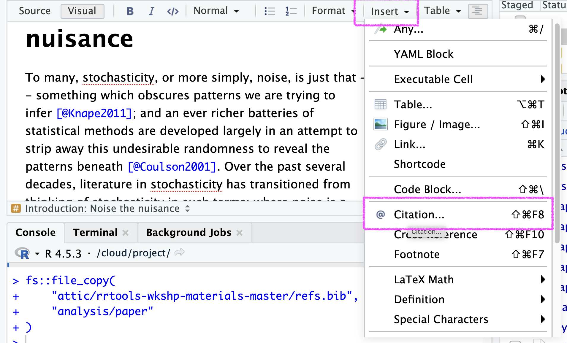
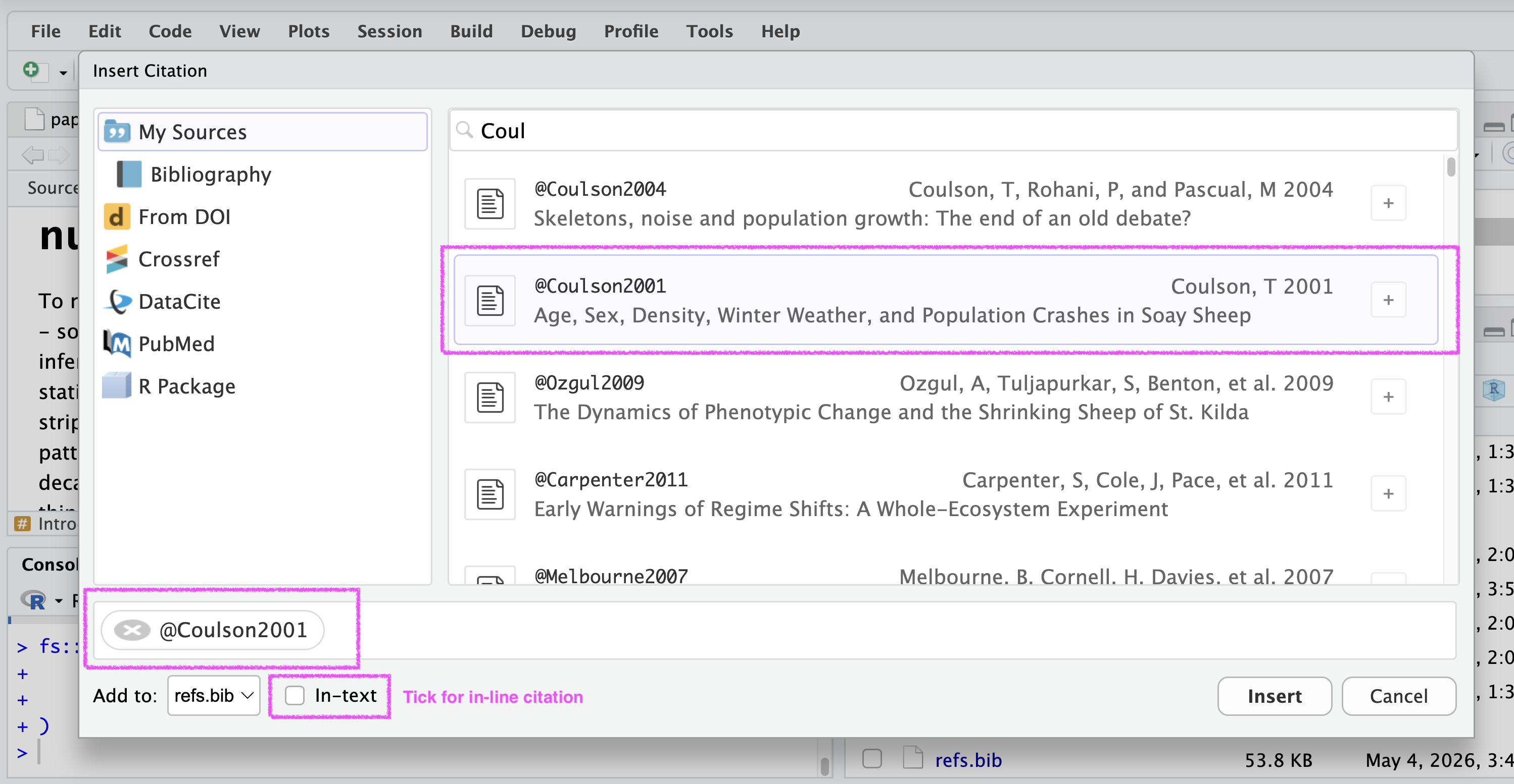
The Insert Citation dialog lets you:
- Search for entries already in your linked bibliography (or in external sources like DOI, Crossref, DataCite, PubMed, R packages) using the source tabs on the left.
- Select one or more entries to insert (multiple citations are allowed).
- Tick In-text to insert as a narrative citation (
Smith (2020)) rather than the default parenthetical form ((Smith 2020)). - The Add to field at the bottom shows which bibliography file the document is linked to (in our case,
refs.bib). Citations imported from external sources get appended there automatically.
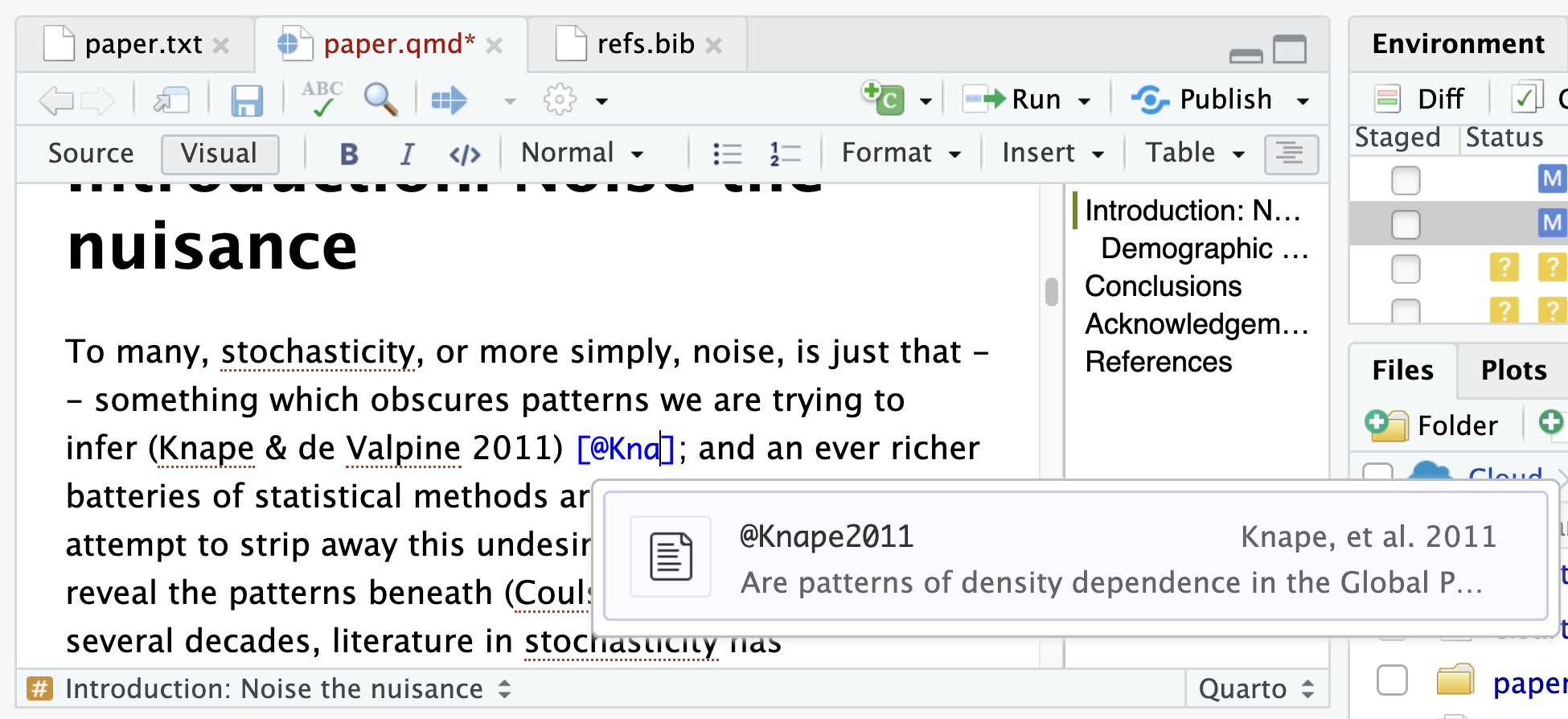
Quicker shortcut (but a bit flaky): typing @ directly in the Visual editor pops up a citation search menu. It’s faster, but the popup can disappear unexpectedly. The Insert > Citation dialog is more reliable.
See the Quarto citations documentation and the Visual editor citation guide for full details.
Once inserted, citation keys appear in the source as [@Knape2011] (parenthetical) or @Knape2011 (in-text). Here’s a snippet of the introduction with three citations inserted:
To many, stochasticity, or more simply, noise, is just that -- something which obscures patterns we are trying to infer [@Knape2011]; and an ever richer batteries of statistical methods are developed largely in an attempt to strip away this undesirable randomness to reveal the patterns beneath [@Coulson2001]. Over the past several decades, literature in stochasticity has transitioned from thinking of stochasticity in such terms; where noise is a nuisance that obscures the deterministic skeleton of the underlying mechanisms, to the recognition that stochasticity can itself be a mechanism for driving many interesting phenomena [@Coulson2004].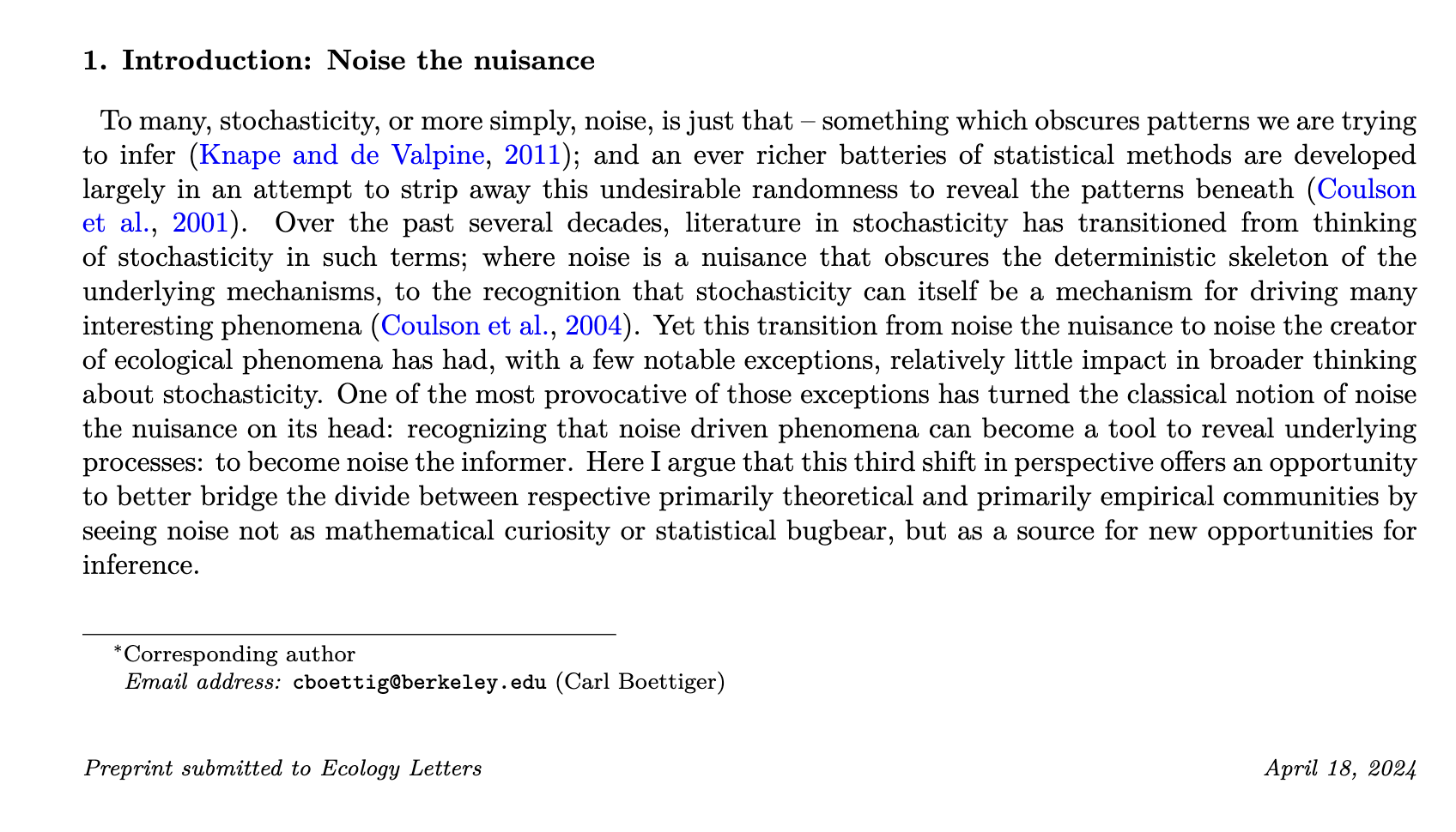
Don’t forget the abstract!
The abstract pasted in earlier also contains a flat citation (Bjørnstad & Grenfell 2001) that needs replacing with the real citation key [@Bjornstad2001].
Interactive citation insertion doesn’t work inside the YAML front matter, so the Insert > Citation dialog and the @ shortcut won’t help here. Just type the [@Bjornstad2001] marker by hand within the abstract: field.
Render analysis/paper/paper.qmd
Click the Render button to see the inline citations correctly formatted and the References section auto-generated at the bottom of the manuscript from the entries in refs.bib.
Commit changes
Add analysis code
Now that we’ve set up the text for our paper, the next step is to add the executable code that generates the figures in the paper. This code is provided in the analysis.R file in the materials we downloaded.
Copy gillespie.csv into project
Before we add the analysis code, let’s copy the data file gillespie.csv from the downloaded materials into analysis/data so the compendium contains its own copy:
fs::file_copy(
  "attic/rrtools-wkshp-materials-master/gillespie.csv",
  "analysis/data"
)
Inspect, edit and run the analysis code
Let’s open attic/rrtools-wkshp-materials-master/analysis.R in the course materials and walk through what it does. The script has some initial setup, then loads the data, recodes one of the columns for plotting, and finally plots the results of the simulation, which generates figure 1 in paper.pdf.
analysis.R
library(dplyr)
library(readr)
library(ggplot2)
library(ggthemes)
theme_set(theme_grey())
# create colour palette
colours <- ptol_pal()(2)

# load-data
data <- read_csv(here::here("gillespie.csv"), col_types = "cdiddd")

# recode-data
data <- data %>%
  mutate(
    system_size = recode(
      system_size,
      large = "A. 1000 total sites",
      small = "B. 100 total sites"
    )
  )

# plot-gillespie
data %>%
  ggplot(aes(x = time)) +
  geom_hline(aes(yintercept = mean), lty = 2, col = colours[2]) +
  geom_hline(aes(yintercept = minus_sd), lty = 2, col = colours[2]) +
  geom_hline(aes(yintercept = plus_sd), lty = 2, col = colours[2]) +
  geom_line(aes(y = n), col = colours[1]) +
  facet_wrap(~system_size, scales = "free_y")
Correct path to data
The script as supplied reads the data with here::here("gillespie.csv"), which expects gillespie.csv to live at the project root. Our copy of gillespie.csv lives in analysis/data/, so we need to update the path in analysis.R to point there:
Run the code
With the path corrected, run the full script. The data loads and the plot is generated:
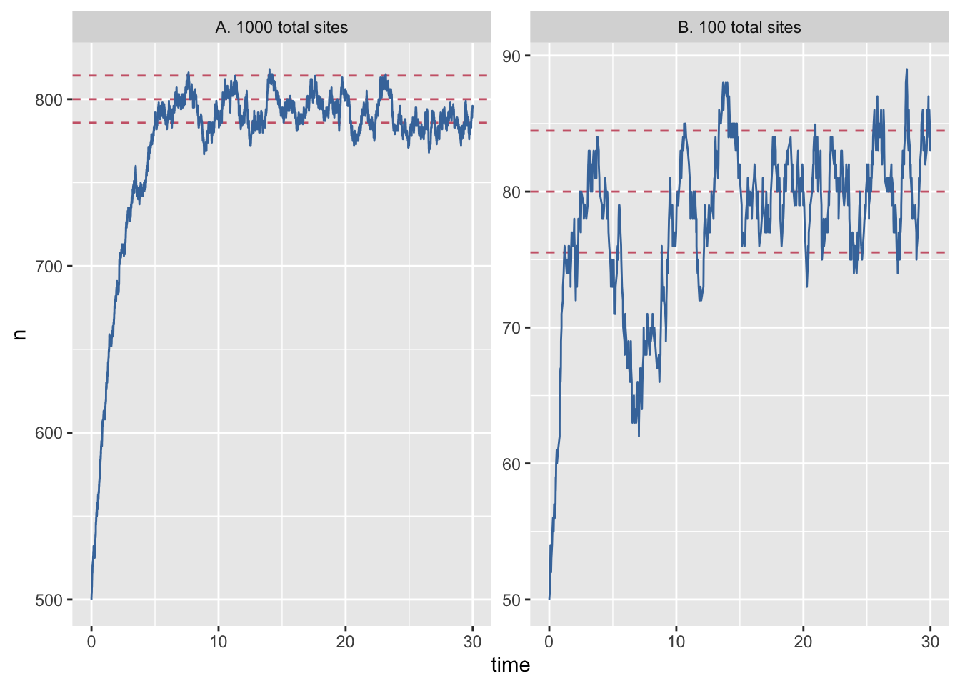
Let’s move back to our paper.qmd file and start adding the code to generate the plot.
Add document level code block configuration
Before we begin, let’s add some document level code block configuration which will apply to all code blocks in our document. We can do this by adding an execute block to bottom of the YAML Front Matter of the paper.qmd file and adding our document level code block settings there.
execute:
echo: false
warning: false
message: falseThis sets the following options for all code blocks in the document:
echo: falsesuppresses the code outputwarning: falsesuppresses warningsmessage: falsesuppresses messages
Add block to load libraries
Next let’s insert a libraries code block right at the top of the document to set up our analysis. Because it’s a set up block we set #| include: false which suppresses all output resulting from block evaluation.
```{r}
#| include: false
#| label: libraries
library(dplyr)
library(readr)
library(ggplot2)
library(ggthemes)
```Add block to set plot themes
Right below the libraries block, insert a new block
Copy the code to set the plot theme and paste it into the block:
```{r}
#| label: set-theme
theme_set(theme_grey())
```Add figure 1 block
Now scroll down towards the bottom of the document and create a new block just above the Conclusions section.
Add code
Paste the analysis code we just ran into the new block:
```{r}
# create colour palette
colours <- ptol_pal()(2)
# load-data
data <- read_csv(
  here::here("analysis", "data", "gillespie.csv"),
  col_types = "cdiddd"
)
# recode-data
data <- data %>%
mutate(system_size = recode(system_size, large = "A. 1000 total sites", small= "B. 100 total sites"))
# plot-gillespie
data %>%
ggplot(aes(x = time)) +
geom_hline(aes(yintercept = mean), lty=2, col=colours[2]) +
geom_hline(aes(yintercept = minus_sd), lty=2, col=colours[2]) +
geom_hline(aes(yintercept = plus_sd), lty=2, col=colours[2]) +
geom_line(aes(y = n), col=colours[1]) +
facet_wrap(~system_size, scales = "free_y")
```Add plot cross-reference
Next, to be able to cross-reference the plot in the text, we need to add a label to the block.
Let’s also add the figure caption found at the bottom of paper.txt to the plot through option fig-cap.
How figure cross-references work in Quarto
Two things turn a chunk’s plot output into a numbered, cross-referenceable figure:
- The chunk
labelmust start with thefig-prefix (e.g.fig-site-simulation). That prefix is what tells Quarto “treat this output as a figure that can be cross-referenced”. - The
fig-capoption supplies the caption text that appears beneath the figure.
With these in place, Quarto auto-numbers the figure and lets you reference it elsewhere in the document with @fig-site-simulation, which renders as a clickable “Figure 1” link.
See the Quarto cross-references docs for the full set of options and prefixes (tbl-, eq-, etc.).
```{r}
#| label: fig-site-simulation
#| fig-cap: "Population dynamics from a Gillespie simulation of the Levins model with large (N=1000, panel A) and small (N=100, panel B) number of sites (blue) show relatively weaker effects of demographic noise in the bigger system. Models are otherwise identical, with e = 0.2 and c = 1 (code in appendix A). Theoretical predictions for mean and plus/minus one standard deviation shown in horizontal re dashed lines."
# create colour palette
colours <- ptol_pal()(2)

# load-data
data <- read_csv(here::here("analysis", "data", "gillespie.csv"),
                 col_types = "cdiddd")

# recode-data
data <- data %>%
  mutate(system_size = recode(system_size, large = "A. 1000 total sites", small= "B. 100 total sites"))

# plot-gillespie
data %>%
  ggplot(aes(x = time)) +
  geom_hline(aes(yintercept = mean), lty=2, col=colours[2]) +
  geom_hline(aes(yintercept = minus_sd), lty=2, col=colours[2]) +
  geom_hline(aes(yintercept = plus_sd), lty=2, col=colours[2]) +
  geom_line(aes(y = n), col=colours[1]) +
  facet_wrap(~system_size, scales = "free_y")
```
Now we can reference this plot in the text using @fig-site-simulation.
So let’s go ahead and replace:
Figure 1 shows the results of two exact SSA simulations of the classic patch modelwith
@fig-site-simulation shows the results of two exact SSA simulations of the classic patch modelwhich will insert a clickable cross-reference to the plot in the text.
Find out more about adding cross-references to code block outputs in the Quarto documentation.
Render analysis/paper/paper.qmd
Click the Render button to see the figure embedded with its caption and the @fig-site-simulation cross-reference resolved as a clickable link in the text. At this point the manuscript is reproducibly generating its own figure from the data in analysis/data/gillespie.csv.
Why
here() is so useful
Notice that the exact same here::here("analysis", "data", "gillespie.csv") path string worked when we ran the corrected analysis.R from the console, and just worked again when the chunk ran from inside analysis/paper/paper.qmd during render, even though the two are in completely different locations in the project.
That’s because here::here() always resolves paths relative to the project root, not the script’s location or your current working directory. So as long as the data file’s location relative to the project root stays constant, the path stays valid no matter where the code is executed from.
This is the convention we set up back in Project Data, Structure & Paths: never hard-code paths and never rely on the working directory; always use here() to keep paths portable.
Commit changes
Update README
Every GitHub repository needs a README landing page.
When we initialised our research compendium, an rrtools README.qmd template was created.
This is one of the real strengths of rrtools: rather than the generic README you’d get from a vanilla R package skeleton, the template contains placeholders tailored specifically for a research compendium, prompting us to fill in:
- authorship and DOI for the associated paper.
- authorship and DOI for the code and data.
- a template citation showing others how to cite your project.
- instructions on how to download and install the compendium.
- instructions on how to reproduce the analysis.
- license information for the text, figures, code and data in your compendium.
The call also created two other community-facing markdown files:
-
CONDUCT.md: a code of conduct for users. -
CONTRIBUTING.md: basic instructions for people who want to contribute to our compendium.
Tip
You can always re-create an rrtools style README with:
rrtools::use_readme_qmd()We need to work through the template and replace its placeholders with information about our project. There are six edits to make:
Set the title
The first chunk in the README contains an R object called Title, used throughout the rest of the document for our paper title. Replace the placeholder string with our actual title:
# Please put your title here to include it in the file below.
Title <- "Partial Reproduction of Boettiger Ecology Letters 2018;21:1255–1267 with rrtools"
Update the project heading
Just below the setup chunk, the README starts with a top-level heading that defaults to the rrtools-generated package name. Update it to match our renamed package:
# rrcompendiumRename master references to main
The template predates the master → main default-branch convention and references it in two places:
- the Binder URL (
...master?urlpath=rstudio→...main?urlpath=rstudio) - the download zip URL (
master.zip→main.zip)
Update file references for Quarto and PDF output
The template defaults assume an R Markdown manuscript rendered to Word. Since we’re using a Quarto manuscript rendered to PDF, update the relevant references:
-
paper.docx→paper.pdf -
paper.Rmd→paper.qmd -
rmarkdown::render("analysis/paper/paper.qmd")→quarto::quarto_render("analysis/paper/paper.qmd")
Adjust the licenses
The template ships with a generic CC-BY-4.0 / CC-0 license block. Update it to match the source compendium’s license (CC-BY-4.0 for everything) and add Carl Boettiger as copyright holder for the text, figures and data we are reusing:
**Text and figures :**  [CC-BY-4.0](http://creativecommons.org/licenses/by/4.0/), Copyright (c) 2018 Carl Boettiger.

**Code :** See the [DESCRIPTION](DESCRIPTION) file

**Data :** [CC-BY-4.0](http://creativecommons.org/licenses/by/4.0/), Copyright (c) 2018 Carl Boettiger.
Render README.qmd
Click the Render button to produce the updated README.md. This is the file GitHub displays as the project landing page, so make sure it reflects all your edits before committing.
Commit changes
Create GitHub repository
Next, we’ll create a GitHub repository to share our compendium.
When working locally, away from the Posit Cloud limitation of all projects being called project, you can use usethis::use_github() to create a new repository on GitHub like we did for our wood-survey project.
# create GitHub repository and push
usethis::use_github()
✔ Creating GitHub repository "annakrystalli/rrcompendium".
✔ Setting remote "origin" to
"https://github.com/annakrystalli/rrcompendium.git".
✔ Adding "https://github.com/annakrystalli/rrcompendium" to URL.
✔ Adding "https://github.com/annakrystalli/rrcompendium/issues" to
BugReports.
ℹ There is 1 uncommitted file:
• DESCRIPTION
! Is it ok to commit it?
1: Nope
2: Negative
3: Yeah
Selection: 3
✔ Adding files.
✔ Making a commit with message "Add GitHub links to DESCRIPTION".
✔ Pushing "main" branch to GitHub and setting "origin/main" as
upstream branch.
✔ Opening URL <https://github.com/annakrystalli/rrcompendium>.This will create a repository on GitHub for our project and push the contents of our project to the main branch of the repository on GitHub. As part of this, use_github() also adds the GitHub repository URL and BugReports links to the DESCRIPTION file and commits that change automatically, so others can easily access the project.
Capture Dependencies
Before we’re finished, let’s ensure the dependencies of our compendium are captured in the DESCRIPTION file so anyone reusing the compendium knows what packages to install.
Declare the development tools
Throughout the workshop we’ve used a handful of development tools to work on the compendium itself: usethis (git/GitHub setup, license, build-ignore, README), credentials (the GitHub PAT) and rrtools itself.
These aren’t needed by paper.qmd to render, but they are needed by anyone who wants to work on the compendium. To make them easy for collaborators to install alongside the analytical dependencies, let’s declare them in a small _dev-deps.R script at the project root:
fs::file_create("_dev-deps.R")Open _dev-deps.R and add the following:
_dev-deps.R
# Development-only dependencies: not used by paper.qmd, but required to
# work on the compendium itself (git/GitHub setup, README, license, etc.).
# Listed here so they get tracked alongside the analytical dependencies in
# DESCRIPTION's Imports field.
library(credentials)
library(usethis)
library(rrtools)
Add _dev-deps.R to the .Rbuildignore so it isn’t bundled into the package itself:
usethis::use_build_ignore("_dev-deps.R")Add analytical dependencies
Now we can use rrtools::add_dependencies_to_description() to automatically detect and record dependencies in the Imports section of DESCRIPTION. The function recursively scans all .R/.qmd/.Rmd files in the project for library() and :: calls, so it will pick up everything from paper.qmd and our new _dev-deps.R in one pass:
rrtools::add_dependencies_to_description()Because rrtools is only available on GitHub (not CRAN), we also need to add a Remotes: field to DESCRIPTION so it can be installed from GitHub. Add this line to your DESCRIPTION:
Remotes: benmarwick/rrtoolsThe Imports and Remotes fields of DESCRIPTION should now look something like this (analytical dependencies plus our three dev tools, with rrtools flagged as a GitHub install):
Imports: here,
    credentials (>= 2.0.2),
    dplyr (>= 1.1.4),
    ggplot2 (>= 3.5.1),
    ggthemes (>= 5.1.0),
    knitr (>= 1.50),
    readr (>= 2.1.5),
    rmarkdown (>= 2.29),
    rrtools (>= 0.1.6),
    usethis (>= 3.1.0)
Remotes: benmarwick/rrtools
and is a good start because it records any packages needed as well as a minimum version required.
To ensure these packages are installed, another user of our project could just run install.packages("remotes") and then remotes::install_deps() to install all the dependencies listed in the DESCRIPTION file.
Initialise project with renv
However, DESCRIPTION alone does not guarantee an exact version of packages, so breaking changes in new versions of packages could cause issues. To ensure exact versions are recorded, we can use renv again to create a snapshot of the project library. In fact we can combine the information contained in the DESCRIPTION file with the snapshot with renv to create an explicit lockfile that tracks the imports listed in DESCRIPTION.
For a refresher on what renv is and the workflow it provides, see Managing R dependencies with renv in the Managing Dependencies chapter, and the renv documentation.
Let’s start by initialising renv in our project.
renv::init()Because it detects a DESCRIPTION file, renv will ask us how to proceed. Select 1: Use only the DESCRIPTION file. (explicit mode).
This project contains a DESCRIPTION file.
Which files should renv use for dependency discovery in this project?

1: Use only the DESCRIPTION file. (explicit mode)
2: Use all files in this project. (implicit mode)
Once selected, renv will proceed to create a lockfile that captures the exact versions of the packages listed in DESCRIPTION in the project library.
- Using 'explicit' snapshot type. Please see `?renv::snapshot` for more details.

- Linking packages into the project library ... [122/122] Done!
The following package(s) will be updated in the lockfile:

# CRAN --------------------------------------------------------
- lattice        [* -> 0.22-6]
- MASS           [* -> 7.3-64]
- Matrix         [* -> 1.7-2]
- mgcv           [* -> 1.9-1]
- nlme           [* -> 3.1-167]

# RSPM --------------------------------------------------------
- base64enc      [* -> 0.1-3]
- bit            [* -> 4.6.0]
- bit64          [* -> 4.6.0-1]
- bslib          [* -> 0.9.0]
- cachem         [* -> 1.1.0]
- cli            [* -> 3.6.4]
- clipr          [* -> 0.8.0]
- colorspace     [* -> 2.1-1]
- cpp11          [* -> 0.5.2]
- crayon         [* -> 1.5.3]
- digest         [* -> 0.6.37]
- dplyr          [* -> 1.1.4]
- evaluate       [* -> 1.0.3]
- fansi          [* -> 1.0.6]
- farver         [* -> 2.1.2]
- fastmap        [* -> 1.2.0]
- fontawesome    [* -> 0.5.3]
- fs             [* -> 1.6.5]
- generics       [* -> 0.1.3]
- ggplot2        [* -> 3.5.1]
- ggthemes       [* -> 5.1.0]
- glue           [* -> 1.8.0]
- gtable         [* -> 0.3.6]
- here           [* -> 1.0.1]
- highr          [* -> 0.11]
- hms            [* -> 1.1.3]
- htmltools      [* -> 0.5.8.1]
- isoband        [* -> 0.2.7]
- jquerylib      [* -> 0.1.4]
- jsonlite       [* -> 1.9.1]
- knitr          [* -> 1.50]
- labeling       [* -> 0.4.3]
- lifecycle      [* -> 1.0.4]
- magrittr       [* -> 2.0.3]
- memoise        [* -> 2.0.1]
- mime           [* -> 0.13]
- munsell        [* -> 0.5.1]
- pillar         [* -> 1.10.1]
- pkgconfig      [* -> 2.0.3]
- prettyunits    [* -> 1.2.0]
- progress       [* -> 1.2.3]
- purrr          [* -> 1.0.4]
- R6             [* -> 2.6.1]
- rappdirs       [* -> 0.3.3]
- RColorBrewer   [* -> 1.1-3]
- readr          [* -> 2.1.5]
- renv           [* -> 1.1.4]
- rlang          [* -> 1.1.5]
- rmarkdown      [* -> 2.29]
- rprojroot      [* -> 2.0.4]
- sass           [* -> 0.4.9]
- scales         [* -> 1.3.0]
- stringi        [* -> 1.8.4]
- stringr        [* -> 1.5.1]
- tibble         [* -> 3.2.1]
- tidyselect     [* -> 1.2.1]
- tinytex        [* -> 0.56]
- tzdb           [* -> 0.5.0]
- utf8           [* -> 1.2.4]
- vctrs          [* -> 0.6.5]
- viridisLite    [* -> 0.4.2]
- vroom          [* -> 1.6.5]
- withr          [* -> 3.0.2]
- xfun           [* -> 0.51]
- yaml           [* -> 2.3.10]

The version of R recorded in the lockfile will be updated:
- R              [* -> 4.4.3]

- Lockfile written to "/cloud/project/renv.lock".
What
renv::init() just created
Our project now contains the infrastructure that powers renv dependency management:
.
├── .Rprofile
├── renv
│   ├── activate.R
│   ├── library
│   │   └── R-4.5
│   │       └── x86_64-pc-linux-gnu
│   └── settings.json
└── renv.lock-
renv.lock: the lockfile, listing the exact version and source of every package in the project library (and the R version it was snapshotted under). -
.Rprofile(andrenv/activate.R): activation hooks that point new R sessions in this project at the project library instead of your user library. -
renv/library/: the project-specific package library. This is never committed to git (renv has already added it to.gitignore).
We commit the rest (renv.lock, .Rprofile and renv/activate.R) so collaborators (and future-you) can reconstruct the same library from the lockfile.
Adjust installation instructions in README
Now that the project uses renv, we need to update the README so anyone who downloads the compendium knows how to set up the project library. The default rrtools template tells them to run devtools::install(), which only installs whatever versions of packages are currently on CRAN: that defeats the point of having a lockfile.
In README.qmd, find the bullet under “How to run in your browser or download and run locally” that currently reads:
- run `devtools::install()` to ensure you have the packages this analysis depends on
  (also listed in the [DESCRIPTION](/DESCRIPTION) file).
Replace it with:
- run `renv::restore()` to install the exact package versions recorded in `renv.lock`.
  You may need to install `renv` first with `install.packages("renv")`.
renv::restore() reads the lockfile and installs each recorded package at the exact version captured in renv.lock, including pulling rrtools from GitHub via the Remotes: line we added earlier. This means collaborators reproduce the same library that produced our results, rather than whatever happens to be the latest on CRAN.
Re-render README.qmd to update README.md.
Commit changes and push to GitHub
Final Compendium
You can browse a demo of the final compendium here
Recap
In this chapter you learnt how to:
-
Scaffold a research compendium with
rrtoolson top of R package conventions. - Combine narrative, code and citations in a single Quarto manuscript using a journal template.
-
Make analysis code reproducible by keeping data in the project and using
here()for portable paths. - Share the compendium on GitHub with appropriate metadata, README and licenses.
-
Capture dependencies in
DESCRIPTIONand pin exact versions withrenvso others can reproduce the same computational environment.
Next topics to explore
Learn more about
renvLearn more about using
rrtoolswith Docker-
Learn more about Binder