
Creating metadata with dataspice
Metadata
The goal of this section is to provide a practical exercise in creating metadata for an example field collected data product using package dataspice.
Understand basic metadata and why it is important.
Understand where and how to store them.
Understand how they can feed into more complex metadata objects.
dataspice workflow
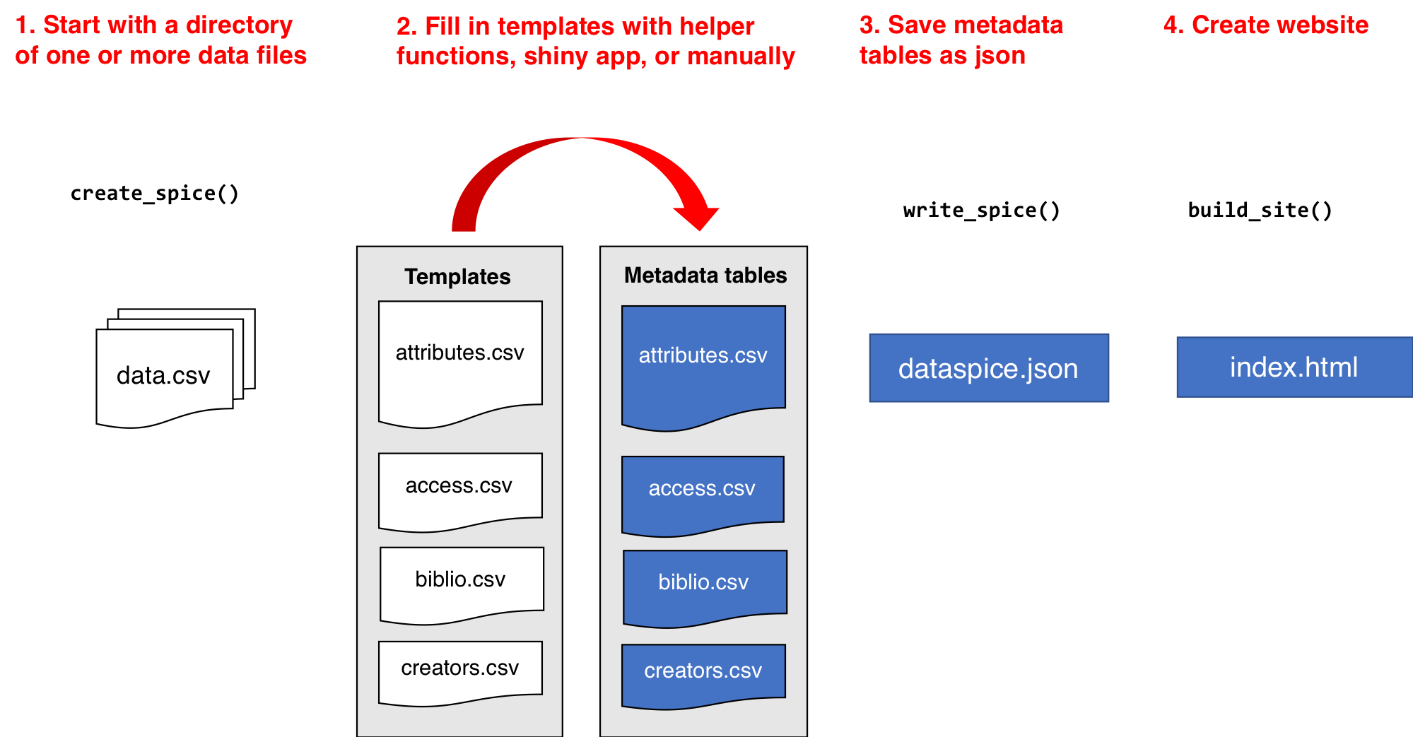
Let’s work in our attic/development.R script for now. The code we use to create our metadata populates files that are part of the project, but the code itself is one-off setup, not part of our analytical pipeline the way data-raw/individual.R and R/geolocate.R are. Keeping it in attic/development.R makes that distinction clear.
Let’s load our library and start creating some metadata! Let’s also load dplyr which we’ll use to extract and collect some metadata programmatically.
Create the metadata folder
We’ll start by creating the basic metadata .csv files in which to collect metadata related to our example dataset using function dataspice::create_spice().
This creates a metadata folder in your project’s data folder by default (although you can specify a different directory if required) containing 4 .csv files in which to record your metadata.
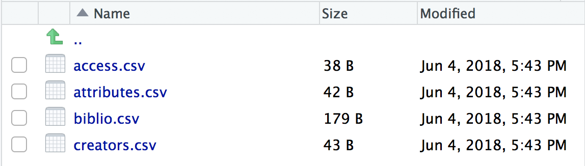
- access.csv: record details about where your data can be accessed from.
- attributes.csv: record details about the variables in your data.
- biblio.csv: record dataset level metadata like title, description, licence and spatial and temoral coverage.
- creators.csv: record creator details.
Record metadata
creators.csv
The
creators.csvcontains details of the dataset creators.
Let’s start with a quick and easy file to complete, the creators. We can open and edit the file using in an interactive shiny app using dataspice::edit_creators().
Although we did not collect this data, just complete with your own details for the purposes of this tutorial.
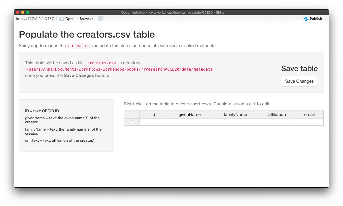
Remember to click on Save when you’re done editing.
access.csv
The
access.csvcontains details about where the data can be accessed.
Before manually completing any details in the access.csv, we can use dataspice’s dedicated function prep_access() to extract relevant information from the data files themselves.
Next, we can use function edit_access() to view and edit access.csv.
The final details required, namely the URL at which each dataset can be downloaded from cannot be completed now so just leave that blank for now.
Eventually it should link to a permanent identifier from which the published data set can be downloaded from.
We can also edit details such as the name field to something more informative if required.
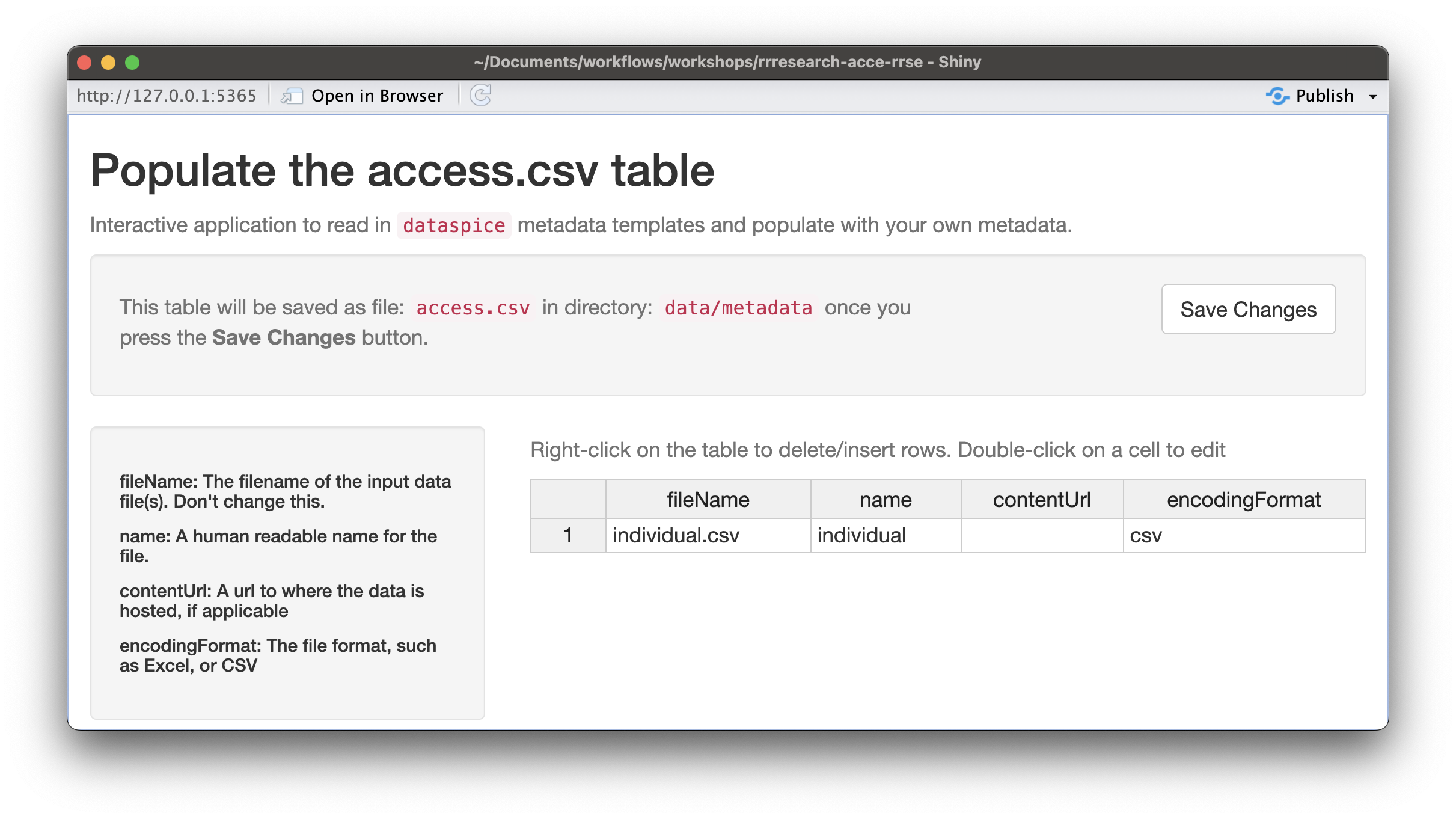
Remember to click on Save when you’re done editing.
biblio.csv
The
biblio.csvcontains dataset level metadata like title, description, licence and spatial and temporal coverage.
Before we start filling this table in, we can use some base R functions to extract some of the information we require. In particular we can use function range() to extract the temporal and spatial extents of our data from the columns containing temporal and spatial data.
Let’s load our data.
get temporal extent
Although dates are stored as a text string, because they are in ISO format (YYYY-MM-DD), sorting them results in correct chronological ordering. If your temporal data is not in ISO format, consider converting them (see package lubridate)
range(individual$date)[1] "2015-05-18" "2018-11-16"get geographical extent
The lat/lon coordinates are in decimal degrees which again are easy to sort or calculate the range in each dimension.
South/North boundaries
range(individual$decimal_latitude)[1] 17.95570 47.16582West/East boundaries
range(individual$decimal_longitude)[1] -99.11107 -66.82463NB: you can also supply the geographic boundaries of your data as a single well-known text string in field wktString instead of supplying the four boundary coordinates.
Geographic description
We’ll also need a geographic textual description.
Let’s check the unique values in domain_id and use those to create a geographic description.
unique(individual$domain_id)[1] "D01" "D02" "D03" "D04" "D07" "D08" "D09"We could use NEON Domain areas D01:D09 for our geographic description.
Now that we’ve got the values for our temporal and spatial extents and decided on the geographic description, we can complete the rest of the fields in the biblio.csv file using function dataspice::edit_biblio().
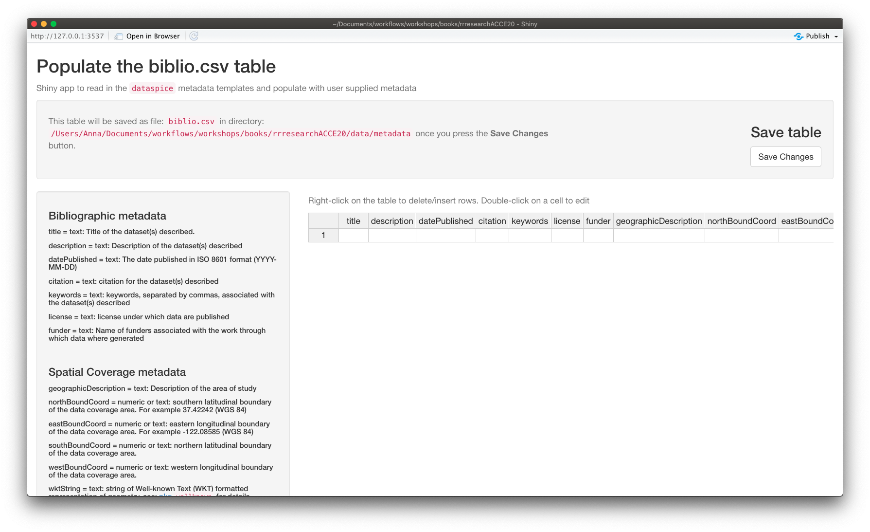
🔍 metadata hunt
Complete the rest of the fields in biblio.csv
Additional information required to complete these fields can be found on the NEON data portal page for this dataset and the data-raw/wood-survey-data-masterREADME.md
Citation: National Ecological Observatory Network. 2020. Data Products: DP1.10098.001. Provisional data downloaded from http://data.neonscience.org on 2020-01-15. Battelle, Boulder, CO, USA
Remember to click on Save when you’re done editing.
attributes.csv
The
attributes.csvcontains details about the variables in your data.
Again, dataspice provides functionality to populate the attributes.csv by extracting the variable names from our data file using function dataspice::prep_attributes().
The functions is vectorised and maps over each .csv file in our data/ folder.
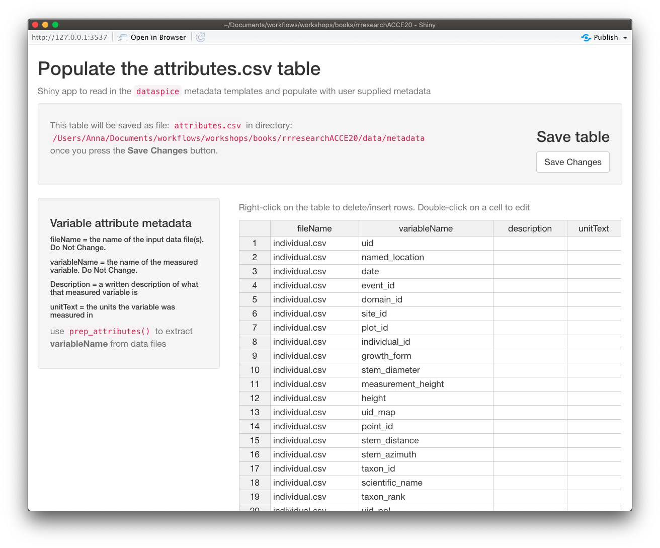
All column names in individual.csv have been successfully extracted as values in the variableName column.
Now, we could manually complete the description and unitText fields,… or we can use a secret weapon, NEON_vst_variables.csv in our raw data!
Let’s read it in and have a look:
variables <- readr::read_csv(
  here::here(
    "data-raw",
    "wood-survey-data-master",
    "NEON_vst_variables.csv"
  ),
  show_col_types = FALSE
)

variables
All original data variable names are contained in fieldName.
variables$fieldName [1] "uid" "namedLocation"
[3] "date" "eventID"
[5] "domainID" "siteID"
[7] "plotID" "subplotID"
[9] "nestedSubplotID" "groupID"
[11] "taxonID" "scientificName"
[13] "taxonRank" "identificationReferences"
[15] "identificationQualifier" "volumePercent"
[17] "livePercent" "deadPercent"
[19] "canopyArea" "meanHeight"
[21] "remarks" "measuredBy"
[23] "recordedBy" "dataQF"
[25] "uid" "namedLocation"
[27] "date" "eventID"
[29] "domainID" "siteID"
[31] "plotID" "subplotID"
[33] "individualID" "tempShrubStemID"
[35] "tagStatus" "growthForm"
[37] "plantStatus" "stemDiameter"
[39] "measurementHeight" "height"
[41] "baseCrownHeight" "breakHeight"
[43] "breakDiameter" "maxCrownDiameter"
[45] "ninetyCrownDiameter" "canopyPosition"
[47] "shape" "basalStemDiameter"
[49] "basalStemDiameterMsrmntHeight" "maxBaseCrownDiameter"
[51] "ninetyBaseCrownDiameter" "remarks"
[53] "recordedBy" "measuredBy"
[55] "dataQF" "uid"
[57] "namedLocation" "date"
[59] "domainID" "siteID"
[61] "plotID" "plotType"
[63] "nlcdClass" "decimalLatitude"
[65] "decimalLongitude" "geodeticDatum"
[67] "coordinateUncertainty" "easting"
[69] "northing" "utmZone"
[71] "elevation" "elevationUncertainty"
[73] "eventID" "samplingProtocolVersion"
[75] "treesPresent" "treesAbsentList"
[77] "shrubsPresent" "shrubsAbsentList"
[79] "lianasPresent" "lianasAbsentList"
[81] "nestedSubplotAreaShrubSapling" "nestedSubplotAreaLiana"
[83] "totalSampledAreaTrees" "totalSampledAreaShrubSapling"
[85] "totalSampledAreaLiana" "remarks"
[87] "measuredBy" "recordedBy"
[89] "dataQF" "uid"
[91] "namedLocation" "date"
[93] "eventID" "domainID"
[95] "siteID" "plotID"
[97] "subplotID" "nestedSubplotID"
[99] "pointID" "stemDistance"
[101] "stemAzimuth" "recordType"
[103] "individualID" "supportingStemIndividualID"
[105] "previouslyTaggedAs" "samplingProtocolVersion"
[107] "taxonID" "scientificName"
[109] "taxonRank" "identificationReferences"
[111] "morphospeciesID" "morphospeciesIDRemarks"
[113] "identificationQualifier" "remarks"
[115] "measuredBy" "recordedBy"
[117] "dataQF" Notice anything inconsistent when you compare the values with those in variableName in attributes.csv? hint: a hump!
Yes you guessed it, the original fieldNames are still in camelCase.
But! variables also contains complete description and units columns! Just what we need!
Now let’s have another look at what our attributes.csv looks like at this point. prep_attributes() has filled in fileName and variableName, but the description and unitText columns are still empty:
Take a moment to compare the two tables side-by-side. There are two things to think about as you look:
- The columns we’d use as join keys (the ones holding the values we want to match on): how do they relate across the two tables?
- The columns we want to bring across into
attributes(the ones with the information we want to populate it with): how do they relate to the columnsattributes(anddataspice) expects?
Mega-Challenge!! 🔍
Your challenge is to populate the description and unitText fields of attributes.csv using the matching information from variables, and save the result back to data/metadata/attributes.csv.
The column structure of attributes.csv must not change. dataspice expects exactly those four columns (fileName, variableName, description, unitText) to build downstream materials from the metadata files. So whatever pipeline you build, the file you save at the end has to have the same column names as the one you started with.
This pulls together most of the verbs you’ve met across day 2: read_csv / write_csv, mutate, select, left_join, rename. A couple of things to think about:
Compare the two tables side-by-side. Look at the column names and at the values in the columns we’d want to join on. Both differ.
Remember our first join, where joining
maptagintoindividualleft us withuid.x/uid.yandeventID.x/eventID.ycolumns? We dealt with that by dropping the unwanted columns from one of the tables before the join (select(maptag, -eventID)). The same thinking applies here.-
The join itself is the new wrinkle. Because the columns we want to match on have different names, you can’t just say
by = "...". Use the modern helperdplyr::join_by()instead, which lets you write the matching rule directly:join_by(x_col == y_col)says “match rows wherex_colfrom the left table equalsy_colfrom the right”. It also opens the door to richer joins (inequality, rolling, overlap) once you need them; see?dplyr::join_by.
One last thing to remember. A couple of the columns in attributes are ones we added ourselves with our get_stem_location() function, so they don’t appear anywhere in NEON’s variables table and will be left with empty description and unitText after your join. Once you’ve completed your merge and saved the file, use dataspice::edit_attributes() to fill those rows in by hand. Their description and unitText will be very similar to those of the plot geolocation variables already in the table, so have a look at those for inspiration.
Create metadata json-ld file
Now that all our metadata files are complete, we can compile it all into a structured dataspice.json file in our data/metadata/ folder.
To do so we use function write_spice().
We can read the dataspice.json file into R as a list using the jsonlite function read_json() and then inspect it using the listviewer package funtion jsonedit.
Publishing this file on the web means it will be indexed by Google Datasets search! 😃 👍
Build metadata site
Finally, we can use the dataspice.json file we just created to produce an informative HTML metadata summary page to include with our dataset for humans to enjoy online! 🤩
We use function dataspice::build_site() which creates an index.html file summarising our metadata. By default it writes to docs/index.html, but we override that with out_path = "data/index.html" so the metadata site lives alongside the data it describes, in our data/ folder (which build_site() will create if it doesn’t already exist).
build_site(out_path = "data/index.html")View the resulting file here
Here’s a screen shot!
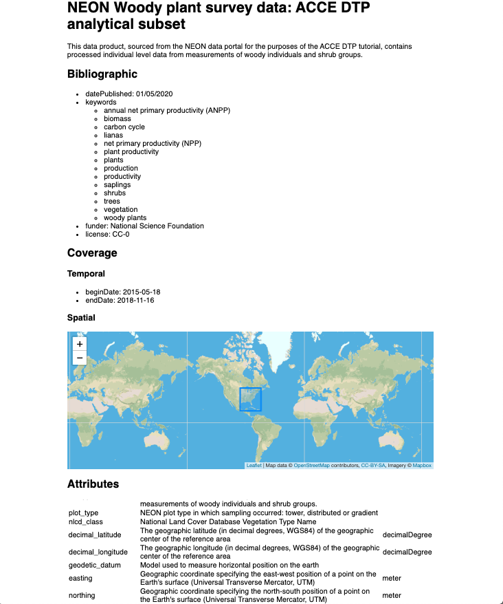
Example completed metadata files
back to the outro slides